Methods for simulation of radiation damage production and evolution
510 likes | 900 Vues
Methods for simulation of radiation damage production and evolution. L. Malerba. Outline. Radiation damage as a multiscale problem Models and techniques to simulate radiation damage production and evolution Neutron-matter interaction Binary collision approximation Molecular dynamics

Methods for simulation of radiation damage production and evolution
E N D
Presentation Transcript
MatGenIV-2 “From iron to steel” – The Ice Hotel, Jukkasjärvi , Sweden, 2-7 Feb 2009 Methods for simulation of radiation damage production and evolution L. Malerba
Outline • Radiation damage as a multiscale problem • Models and techniques to simulate radiation damage production and evolution • Neutron-matter interaction • Binary collision approximation • Molecular dynamics • Atomistic Monte Carlo models • Metropolis Monte Carlo • Atomistic kinetic Monte Carlo • Coarse-grained microstructure evolution models • Rate theory • Object kinetic Monte Carlo • Summary • The problem of the “experimental validation” MatGenIV-2 “From iron to steel” – The Ice Hotel, Jukkasjärvi , Sweden, 2-7 Feb 2009 – L. Malerba - Simulation
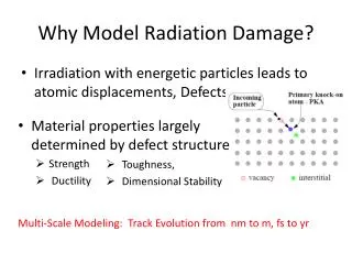
ns = 10-9 s ….. ms = 10-3 s ….. 1 s …… 103 s 1 fs = 10-15 s 1-100 ps = 10-12- 10-10 s Time scale Precipitates Loops &Cavities Displacement Cascade Cascade ageing Cascade accumulation Primary state of damage Relaxation Thermal spike Collisions From n spectrum to PKA & Displacement Cascade Spectrum Inciedent particles Nucleation & Growth of Precipitates & Large Clusters Secondary Defect Formation Defect Migration Length scale hundreds of nm = 10-7 m tens of nm = 10-8 m Radiation effects are inherently multiscale and multiphysics phenomena Louvain-la-neuve, 15 Dec 2008 – L. Malerba
s = 10-3 s.........................…………………….…… Years = 107 -109 s Time scale Cascade accumulation Growing Concentration of Radiation Induced Defects while the Irradiation Proceeds applied shear Dislocation pinning pinned dislocation Mechanical Property Changes Failure Irradiated Dislo/Defect Interaction Yield Strength Increase Stress (MPa) Unirradiated Length scale Strain (%) cm = 10-2 m tens of m = 10-5 m Radiation effects are inherently multiscale and multiphysics phenomena Louvain-la-neuve, 15 Dec 2008 – L. Malerba
Multiscale modelling tools • Different computer simulation tools exist to study the different phases of radiation damage • Each of them is the result of long algorithm development work, started already between the 50s and 70s • The practical widespread implementation of these algorithms dates mainly from the late 80s – early 90s • In what follows, a bird’s eye view on the most important of these is provided MatGenIV-2 “From iron to steel” – The Ice Hotel, Jukkasjärvi , Sweden, 2-7 Feb 2009 – L. Malerba - Simulation
N (at·cm-3·s-1) (n·cm-2·s-1) Recoil spectrum Neutron spectrum 10 MeV E (MeV) E (MeV) 1 MeV Nuclear cross-section library (e.g. ENDF/B-V) Electronic excitation fraction, dpa NRT, … Neutron-Matter Interaction Neutron transport codes like SPECTER calculate the recoil spectrum for a given neutron spectrum – the reliability of the code depends ultimately on the reliability of the library of nuclear cross-sections MatGenIV-2 “From iron to steel” – The Ice Hotel, Jukkasjärvi , Sweden, 2-7 Feb 2009 – L. Malerba - Simulation
Cascades: Binary Collision Approximation • Particle trajectories built as series of binary encounters between projectiles and stationary atoms: • Direction changes are results of collisions, treated with basic kinematics conservation laws • Between collisions particles move along asympthotic paths • Material represented by displacement energies, binding energies, recombination radii • High energy recoils are easily simulated within fractions of seconds • The method cannot treat many-body interactions at thermal equilibrium, nor provide actual defect configurations at atomic-level MatGenIV-2 “From iron to steel” – The Ice Hotel, Jukkasjärvi , Sweden, 2-7 Feb 2009 – L. Malerba - Simulation
Molecular Dynamics • Principle • The classical equations of motion for a set of N atoms are timestepwise solved, using finite difference integration algorithms, so as to know atomic positions and velocities at each timestep: • From the knowledge of atomic positions and momenta all atomic-level and also statistical mechanics quantities are directly accessible • The core of the method, containing all the physics, is the interatomic potential, V(ri),from which the interatomic forces are derived MatGenIV-2 “From iron to steel” – The Ice Hotel, Jukkasjärvi , Sweden, 2-7 Feb 2009 – L. Malerba - Simulation
Molecular Dynamics • Atoms are distributed in a simulation box, in initial positions corresponding to a crystal lattice • Initial velocities are randomly assigned, according to temperature • Periodic boundary conditions simulate the infinite crystal MatGenIV-2 “From iron to steel” – The Ice Hotel, Jukkasjärvi , Sweden, 2-7 Feb 2009 – L. Malerba - Simulation
Molecular dynamics for cascades • MD is the technique “par excellence” for displacement cascade simulations: • one atom is given a kinetic energy of a few keV to tens of keV • the dynamical evolution of the system is followed • the ballistic phase (BCA) is spontaneously reproduced • the equilibrium defect configurations are also correctly treated, compatibly with the validity of the potential 5 keV cascade (peak time) in SiC MatGenIV-2 “From iron to steel” – The Ice Hotel, Jukkasjärvi , Sweden, 2-7 Feb 2009 – L. Malerba - Simulation
Molecular dynamics for defect studies • Diffusion studies • Single point defects • vacancies at high T • self-interstitial atoms – SIA – at any temperature • SIA clusters • vacancy clusters are too slow for MD • Reactions between defects • Formation of SIA clusters by absorption of single SIA • Coalescence of SIA clusters • … Courtesy D. Terentyev MatGenIV-2 “From iron to steel” – The Ice Hotel, Jukkasjärvi , Sweden, 2-7 Feb 2009 – L. Malerba - Simulation
Molecular dynamics for dislocation/defect interaction studies In the last 10 years the development of models of radiation-induced hardening has been addressed by studying in detail by MD the interaction between dislocations and radiation-produced defects Courtesy of D. Terentyev MatGenIV-2 “From iron to steel” – The Ice Hotel, Jukkasjärvi , Sweden, 2-7 Feb 2009 – L. Malerba - Simulation
Advantages Wide applicability (bulk, surfaces, crystals, amorphous, liquids, ...) No analytical simplifications or approximations Treats spontaneously complex systems and phenomena at equilibrium or far from it, not accessible to analytical approaches Provides information about atomic-level configurations and mechanisms Allows characteristic energies and other key quantities not accessible to experiments to be assessed Limitations Limited timescale (tens of nanoseconds, trade-off size/time) Limited volumes (up to 107 atoms): not big enough for e.g. extended defects All the physics is contained in the interatomic potential: the validity of the results depends totally on the ability of the interatomic potential to reproduce the behaviour of the material studied Pros & Cons of MD MatGenIV-2 “From iron to steel” – The Ice Hotel, Jukkasjärvi , Sweden, 2-7 Feb 2009 – L. Malerba - Simulation
Stochastic Monte Carlo Algorithms • Molecular dynamics cannot deterministically reproduce the evolution of a system to equilibrium if the kinetics is slower than nanoseconds • Monte Carlo methods can be used for this purpose or more generally to extend the timespan of radiation damage simulations: • Metropolis Monte Carlo • Kinetic Monte Carlo • Atomistic KMC • Object KMC MatGenIV-2 “From iron to steel” – The Ice Hotel, Jukkasjärvi , Sweden, 2-7 Feb 2009 – L. Malerba - Simulation
P1 P2 Pi Pk PN 0 1 The Monte Carlo Algorithm • List of possible events: ei / i=1, …, Ne • A probability Pi is associated to each event • iPi = 1 • Monte Carlo step: ek Random number extraction, Rn [0,1] MatGenIV-2 “From iron to steel” – The Ice Hotel, Jukkasjärvi , Sweden, 2-7 Feb 2009 – L. Malerba - Simulation
Metropolis Monte Carlo • System of N atoms, where defects can be included • The total energy must be calculable, e.g. using an interatomic potential (or any other hamiltonian) • One trial event is chosen between: • atomic position exchange • small atomic displacement • global expansion or contraction • If Eafter- Ebefore = E < 0, the trial is accepted • If E > 0, the trial is accepted with probability exp(- E/kT) < 1 (by extracting a random number, which can fall only in one out of two possible probability intervals) MatGenIV-2 “From iron to steel” – The Ice Hotel, Jukkasjärvi , Sweden, 2-7 Feb 2009 – L. Malerba - Simulation
Metropolis Monte Carlo • Useful to study possible least free energy configuration corresponding to a certain atomic composition and/or defect concentration • Phase separation • Segregation of solute atoms at extended defects (GBs, dislocations, …) • Segregation of solute atoms at point-defect clusters • Equilibrium is reached when energy does not change any more after a number of trials: then microstates of same macrostate are sampled Example of application: compare the phase diagram given by an interatomic potential with the experimental phase diagram E. Zhurkin et al., 2008 MatGenIV-2 “From iron to steel” – The Ice Hotel, Jukkasjärvi , Sweden, 2-7 Feb 2009 – L. Malerba - Simulation
Metropolis Monte Carlo Advantages • Phenomena such as segregation or precipitation, out of scope for MD, can be studied • (given a suitable hamiltonian and on the condition that these correspond to equilibrium states) • All contributions to the free energy can be included in the calculation • Powerful tool to evaluate phase diagrams Problems: • Evolution does not involve physical mechanisms, only total energy • Intermediate configurations are physically not meaningful • No information is given about time necessary to reach equilibrium MatGenIV-2 “From iron to steel” – The Ice Hotel, Jukkasjärvi , Sweden, 2-7 Feb 2009 – L. Malerba - Simulation
Kinetic Monte Carlo Kinetic time is introduced ! • Probabilities are calculated for physical transition mechanisms as Boltzmann factor frequencies : • After a certain event is chosen, time is increased by an amount: (residence time algorithm) Most physics (kinetics and thermodynamics) contained in the activation energies ! MatGenIV-2 “From iron to steel” – The Ice Hotel, Jukkasjärvi , Sweden, 2-7 Feb 2009 – L. Malerba - Simulation
Kinetic Monte Carlo Families Atoms (alloy) on rigid lattice Mainly vacancy jumps (SIA in 1st approx.) Energy parameters from interatomic potentials or DFT Atomistic KMC KMC residence time algorithm “Objects” on non-atomic lattice (V, SIA, clusters, …) Many possible reactions between “objects” Large set of parameters covering all possible reactions is needed Object KMC MatGenIV-2 “From iron to steel” – The Ice Hotel, Jukkasjärvi , Sweden, 2-7 Feb 2009 – L. Malerba - Simulation
NEB Emig (eV) DE = Ef - Ei (eV) Atomistic KMC: Heuristic estimates of Ea • Energy difference method E0 Ef Ei • Advantages: • Evolution biased towards lower energy • It does not matter, a priori, how the energy is calculated (interatomic potential, pair-energies, ab initio, …) • Problem: • When the defect jumps, it does not know what the energy will be after the jump! MatGenIV-2 “From iron to steel” – The Ice Hotel, Jukkasjärvi , Sweden, 2-7 Feb 2009 – L. Malerba - Simulation
Atomistic KMC: Heuristic estimates of Ea • Broken-bond applied to saddle point Esp Eini • Advantages: • Somewhat more physical, while still computationally cheap • Limitations: • Energy evaluation can only be done via pair energies fitted to some more fundamental cohesive model: extrapolability? MatGenIV-2 “From iron to steel” – The Ice Hotel, Jukkasjärvi , Sweden, 2-7 Feb 2009 – L. Malerba - Simulation
AKMC: advanced approaches Neural Network Local Atomic Config. (string of integers) Ea* 1 1 2 1 2 1 1 2 1 1 1 2 2 1 1 1 2 1 2 1 N. Castin, 2008 MatGenIV-2 “From iron to steel” – The Ice Hotel, Jukkasjärvi , Sweden, 2-7 Feb 2009 – L. Malerba - Simulation
Example of application of AKMC: precipitation in FeCr G. Bonny et al., Phys. Rev. B, 2008 MatGenIV-2 “From iron to steel” – The Ice Hotel, Jukkasjärvi , Sweden, 2-7 Feb 2009 – L. Malerba - Simulation
AKMC: Pros & Cons • Advantages: • Atomic-level method: can treat diffusion processes including proper atomic level mechanisms • Can be extended to relatively long timescales (it depends on the problem), much longer than MD any way (seconds easily) • Limitations: • Computationally expensive: the volumes that can be simulated remain fairly small • At the moment, the treatment of SIA is only tentative If a reliable and efficient method to calculate barriers on-the-fly for any defect is found and a proper parallelisation scheme is developed, AKMC methods can become competitive and are probably the only way to adequately model radiation damage in concentrated alloys MatGenIV-2 “From iron to steel” – The Ice Hotel, Jukkasjärvi , Sweden, 2-7 Feb 2009 – L. Malerba - Simulation
Coarse-grained microstructure evolution models • Coarse-grained no atoms • The “elements” or “grains” of the simulation are not atoms: • Defects (point-defects, clusters, precipitates) microstructure evolution models • Dislocations dislocation dynamics models • Grain-boundaries texture models • … • Microstructure evolution models for radiation damage are those that in principle allow direct comparison with experiments: • Rate theory • Object kinetic Monte Carlo (and similar) MatGenIV-2 “From iron to steel” – The Ice Hotel, Jukkasjärvi , Sweden, 2-7 Feb 2009 – L. Malerba - Simulation
Microstructure evolution models:Rate Theory • Mean-field approximation: Defects are created, react and disappear at sinks everywhere at the same rate • The same thing happens in each infinitesimal volume dV V • Different from periodic boundary conditions: • dV 0 (infinitesimal) • There is no real simulation volume • Only variables are concentrations dV Source term Flux term Reaction term • Example: MatGenIV-2 “From iron to steel” – The Ice Hotel, Jukkasjärvi , Sweden, 2-7 Feb 2009 – L. Malerba - Simulation
Microstructure evolution models:Rate Theory • N (10s to 100s) coupled differential equations of this type need to be written, one for each defect species • The actual rate theory concerns the determination of the “rates” at which the reactions occur • E.g., through the theory of diffusion-limited reactions and based on mass-action law we know that: • Thus, given the source terms, the basic ingredients of microstructure evolution models are • Diffusion coefficients • Capture radii • Binding energies MatGenIV-2 “From iron to steel” – The Ice Hotel, Jukkasjärvi , Sweden, 2-7 Feb 2009 – L. Malerba - Simulation
Microstructure evolution models:Rate Theory Sink strength k21/l2 mean free path before absorption • Another example: single vacancies and single self-interstitials: • Most important theoretical advances in rate theory concern determination of expressions for sink strenghts • Uniformely distributed spherical absorbers • Dislocation lines (theoretical expression available only for array of infinite parallel dislocation) • Uniformely distributed dislocation loops • Grain boundaries • Sink strengths depend also on migration features • One-dimensional versus three-dimensional • Different of comparable diffusion coefficient MatGenIV-2 “From iron to steel” – The Ice Hotel, Jukkasjärvi , Sweden, 2-7 Feb 2009 – L. Malerba - Simulation
Microstructure evolution models:Rate Theory – Pros & Cons Advantages: • Computationally cheap (if no pbs of solver stability arise …): • Sensitivity studies are easily performed • Fitting of parameters to experiments is possible • Large fluences and volumes are no problem • Steady-state or simplified expressions can be analytically obtained • Fully theoretical framework within which radiation effects can be addressed • It is not a “simulation” • Computer solves system of eqs. Drawbacks: • Random inhomogeneities and geometrical effects (e.g. coalescence) not taken into account • Introduction of new mechanisms requires specific theoretical developments • All acting mechanisms and parameters must be known • The model does not provide them, like e.g. MD • Atomic-level configurations are not provided, either • As compared to e.g. AKMC MatGenIV-2 “From iron to steel” – The Ice Hotel, Jukkasjärvi , Sweden, 2-7 Feb 2009 – L. Malerba - Simulation
Microstructure evolution models:Object kinetic Monte Carlo • Volume containing “objects” exists: • Point-defects and their clusters • Precipitates, solutes, … • Traps and localised sinks • Dislocations • (Grain boundaries) • Each “object” is defined by: • Type • (centre-of-mass) position • Migration parameters • Possible reactions • Reaction radius • Events can be • Thermally activated activation energy (migration, emission) • External of known rate Pi (cascades, …) • Effect of geometry (recombination, trapping, clustering) MatGenIV-2 “From iron to steel” – The Ice Hotel, Jukkasjärvi , Sweden, 2-7 Feb 2009 – L. Malerba - Simulation
Density (m-3) Density (m-3) dpa set 1 set 2 set 3 dpa Microstructure evolution models:Object kinetic Monte Carlo - example PBC 100 ppm SIA traps SIA clusters must be 1D-mobile in Fe But traps must exist to stop some of them MatGenIV-2 “From iron to steel” – The Ice Hotel, Jukkasjärvi , Sweden, 2-7 Feb 2009 – L. Malerba - Simulation
Microstructure evolution models:Object kinetic Monte Carlo: Pros & Cons • Advantages: • Flexibility in introducing objects, mechanisms and parameters, taken from any source of information (DFT, MD, AKMC, experiments, …) • No theoretical developments required for each new mechanism • Spatial inhomogeneities and correlations (including sink strengths) are spontaneously accounted for • Defects behave in a realistic way • Drawbacks: • No atomic configurations • As compared to atomistic KMC • All mechanisms and parameters must be known in advance • The model does not provide them, like MD does • Computationally expensive • (as compared to rate theory) • Small volumes reduce statistical significance, especially for low densities • Fitting not possible; sensitivity studies possible, but at high cost MatGenIV-2 “From iron to steel” – The Ice Hotel, Jukkasjärvi , Sweden, 2-7 Feb 2009 – L. Malerba - Simulation
Comment on microstructure evolution models • OKMC and rate equations share the same problem of requiring all mechanisms and parameters to be known in advance • OKMC is more realistic in terms of spatial correlations, but computationally expensive • RT is computationally cheap, but cannot include spatial effects properly • They are currently considered as complementary tools • However, neither of them can treat at the same time defect evolution and phase changes, especially in concentrated alloys MatGenIV-2 “From iron to steel” – The Ice Hotel, Jukkasjärvi , Sweden, 2-7 Feb 2009 – L. Malerba - Simulation
ns = 10-9 s ….. ms = 10-3 s ….. 1 s …… 103 s 1 fs = 10-15 s 1-100 ps = 10-12- 10-10 s Time scale Precipitates Loops &Cavities Displacement Cascade Molecular dynamics Atomistic and Object kinetic Monte Carlo Relaxation Thermal spike Collisions From n spectrum to PKA & Displacement Cascade Spectrum Neutron transport Nucleation & Growth of Precipitates & Large Clusters Secondary Defect Formation Defect Migration Length scale 100s of nm = 10-7 m 10s of nm = 10-8 m Multiscale modelling tools - summary MatGenIV-2 “From iron to steel” – The Ice Hotel, Jukkasjärvi , Sweden, 2-7 Feb 2009 – L. Malerba - Simulation
s = 10-3 s.........................…………………….…… Years = 107 -109 s Time scale Rate theory, Object KMC Growing Concentration of Radiation Induced Defects while the Irradiation Proceeds applied shear Dislocation dynamics pinned dislocation Mechanical Property Changes Failure Irradiated Plasticity models Dislo/Defect Interaction Yield Strength Increase Stress (MPa) Unirradiated Length scale Strain (%) cm = 10-2 m 10s of m = 10-5 m Multiscale modelling tools - summary MatGenIV-2 “From iron to steel” – The Ice Hotel, Jukkasjärvi , Sweden, 2-7 Feb 2009 – L. Malerba - Simulation
Small Angle Neutron Scattering Tomographic Atom Probe Electron Microscopy: (HR)TEM, FEGSTEM, … Combination of advanced experimental techniques Positron Annihilation Internal Friction Experimental validation Comparison with models The comparison is not simple, though! MatGenIV-2 “From iron to steel” – The Ice Hotel, Jukkasjärvi , Sweden, 2-7 Feb 2009 – L. Malerba - Simulation
“Experimental validation” Build a picture: Simulation results Monte Carlo result Ab initio results MD results ? MatGenIV-2 “From iron to steel” – The Ice Hotel, Jukkasjärvi , Sweden, 2-7 Feb 2009 – L. Malerba - Simulation
“Experimental validation” Build a picture: Experimental result ??? MatGenIV-2 “From iron to steel” – The Ice Hotel, Jukkasjärvi , Sweden, 2-7 Feb 2009 – L. Malerba - Simulation
“Experimental validation” God-like view MatGenIV-2 “From iron to steel” – The Ice Hotel, Jukkasjärvi , Sweden, 2-7 Feb 2009 – L. Malerba - Simulation
MatGenIV-2 “From iron to steel” – The Ice Hotel, Jukkasjärvi , Sweden, 2-7 Feb 2009 The End