Download
1 / 33
330 likes | 507 Vues
Plumes, Ice and the Polar Oceans. Tony Payne, Steph Cornford and Dan Martin* University of Bristol, Lawrence Livermore National Laboratory *. Outline. Introduction on the triggers of change Ice-ocean interactions and buoyant plumes Adaptive-mesh refinement and ice sheets

E N D
Plumes, Ice and the Polar Oceans TonyPayne, StephCornfordand Dan Martin* University of Bristol, Lawrence Livermore National Laboratory *
Outline • Introduction on the triggers of change • Ice-ocean interactions and buoyant plumes • Adaptive-mesh refinement and ice sheets • Projections of the Antarctic contribution to sea level over next 200 years
“… but ... flow rates could increase or decrease in the future.” “Larger values cannot be excluded …” “… understanding of these effects is too limited to assess their likelihood or provide a best estimate or an upper bound for sea level rise.”
Antarctic mass balance from satellites • interior thickening related to changes in snowfall • coastal thinning in WAIS (Pine Island, Smith and Thwaites Glaciers) and EAIS (Cook and Totten Glaciers) • close correspondence to ice velocity (ice streams) Pritchard and others 2009 Shepherd and Wingham 2007
Atmospheric triggers • collapse of Larsen A ice shelf in 1995 and B in 2002 • meltwater-driven fracture understood MacAyeal and others 2003
Atmospheric triggers • minimal direct effect, however glaciers accelerated after collapse • natural experiment testing link between floating and grounded ice 2003/2005 1996/2000 Rignot 2004 Scambos and others 2004
Pritchard and others 2009 Oceanic triggers • observed GL retreat rates consistent with GL occupying ridge in mid 1990s (Jenkins and others (2010) • retreat has been consistent since 1990s and accelerated through 2000s - 0.95 ±0.09 km/yr with peak 2.8 ± 0.7 km/yr 2009 2000 1996 2011 1992 Jenkins and others 2010 Park and others (accepted)
Oceanic triggers 1995 Wingham and others (2009) use cross-calibrated ERS-2 and ENVISAT radar altimetry to extend time series from 1995 to 2008 thinning rates increased fourfold 2006
Oceanic triggers • Jacobs (2006) suggests a mechanism controlling upwelling on to shelf • Circumpolar Deep Water (CDW) is dominant water mass ~ 4 °C above melt point at grounding line • recent cruises to the area indicate that CDW can cross on to continental shelf and under the ice shelf Walker and others 2007 Jenkins and others 2010
ice melt/freeze plume D T,S,U,V entrainment ambient Ice-ocean coupling: plume model • vertically integrated (i.e, 2d), time dependent • mass balance gives plume depth (D) incorporates melt and entrainment • horizontal momentum balances (U and V) (Coriolis, lateral and surface drag, buoyancy etc included) • temperature (T) and salinity (S) transport with lateral mixing • linearized equation of state for density • run to equilibrium in ~ 10 days, 1 km horizontal resolution
33.8 -1.9 34.7 600 m 1.0 CDW Entrainment of ambient water • 1994 profiles of ambient temperature and salinity from Jacobs and others (GRL 1996)
Flow of plume controlled by geometry of ice shelf base Predicted water depth (m) Depth of ice shelf base (m)
Path of plume • predicted outlets coincide with polynas
Melt rate pattern • some agreement with ice-flux divergence • very high close to grounding line • higher in path of plume Predicted m/yr Div. calculation m/yr
Heat budget • non-linear relationship of melt to temperature at high rates • linear for moderate melt rates over bulk of shelf
Heat budget • heat gained by entrainment of warm water • lost in melt • most entrained heat used locally • some used downstream • virtually no net export
Implications • melt rates predicted to vary spatially • pattern controlled by details of ice-shelf geometry • possible interactions between steeper ice, faster velocities in plume and greater entrainment/melt • positive feedback moderated by flow of ice shelf Depth of ice shelf base (m)
Modelling grounding line migration • Durand and others (2009) and Vieli and Payne (2005) show fixed grids models can generate robust solution but require higher order physics and very fine resolution (sub km) • major challenge to provide sub-km resolution for whole ice sheet (14×106 km2 ) • one solution is adaptive mesh refinement
Bisicles ice sheet model • Specifically designed for GL problems • Based on CHOMBO adaptive-mesh refinement developed by Lawrence Livermore National Lab. • CHOMBO ensures conservation between grids and offers massive parallelization
gravitational driving normal stress deviators horiz. shear stresses Bisicles • Uses a vertically-integrated form of the stress equations proposed by Schoof and Hindmarsh (2010) known as L1L2 • Similar to ‘shelfy’ stream except that effective viscosity (f) includes a representation of the vertical structure of the flow (i.e., does not assume ‘plug’ flow) • Solved using CHOMBO’s multigrid library making use of a Jacobian-free Newton-Krylov method basal traction
BISICLES • Trial application to Pine Island Glacier • Simulation using reasonable melt increase of 50 m/yr • Results dependent on resolution from single level (5km) to six levels (~150 m) • Confirms need for sub-km resolution Colours refer to velocity
Sea level projections • Coupled problem but no such coupled model exists • Use a chain of models from global AOGCMs regional ocean and atmosphere models ice sheet model • Consider only West Antarctica
SRES scenarios A1B and E1 with AOGCMS Experimental design HadCM3 ECHAM5 Snowfall - regional atmospheric modelling Melt - regional ocean modelling RACMO2 (Utrecht) LMDZ4 (Grenoble) E1 BRIOS (AWI) FESOM (AWI) Anomalies against 1980 to 1989 BISICLES ice sheet model
Snowfall forcing Sea level fall Anomalies from two RCMs are fairly consistent HadCM3 forcing produces ~2 times ECHAM5 for A1B but very similar for E1 A1B 20-30% incr. E1 5-10% incr. Baselines are 1900 Gt/yr for RACMO2 and 2800 Gt/yr for LMDZ4
Ocean forcing – major ice shelves • Warm water intrusion reported by Hellmer and others (2012) for BRIOS also in FESOM for Ronne-Filchner • Leads to 10-20 fold increase in melt • Similar phenomenon for Ross ice shelf after 2100 (FESOM only) Ronne-Filchner ice shelf Ross ice shelf
Ocean forcing – smaller ice shelves • FESOM and BRIOS do not represent smaller shelves well • Use index of coastal warming and convert to melt anomaly using empirical relation (e.g., Jacobs and Rignot 2002) • Warming of 1 to 2 C or 10-20 m/yr Jacobs and Rignot 2002
Derived basal traction coeff. Initial conditions • Observed ice sheet geometry • Use methods based on Lagrange multipliers to find ice viscocity and basal traction consistent with observed velocities • Evolve ice sheet for 50 years to allow noise to relax away Derived rheology factor
Results • Background is the initial velocity field • KEY - • 1980 ground line • Worst case by 2200 • Control (no anomalies) shows some drift
Filchner-Ronne ice shelf • Strong imposed melt sufficient to melt holes in the ice shelf • Widespread GL retreat by 2200 of ~100 km • Roughly balances increased snowfall until after 2150 • E1 greater SLR than A1B! Control Ocean only
Ross ice shelf • Retreat in lightly grounded areas even in control • In general, increased accumulation dominates Control Ocean only
Amundsen Sea and Pine Island • Deglaciation of Pine Island Glacier and Smith Glaciers • Thwaites shows no retreat related to lack of buttressing? • Similar to recent GL observations • In general, increased accumulation dominates Pine Island Glacier Thwaites Glacier Smith Glacier
Summary • Increased outflow is enough to compensate increased snowfall • Sea level rise is predicted as -5 to 80 mm by 2200 depending on forcing (i.e., small) • Sea level rise is limited because • GL retreat occurs late in the model run (c.f. ocean forcing) • Areas that retreat do not have much ice above buoyancy (so little effect or SLR) and/or • Large retreat limited to narrow channels (e.g., Pine Island) • Sea level rise appears to continue to increase beyond 2200 • Omits East Antarctica • Fuller estimate requires coupling to regional ocean model