Download

1 / 41
410 likes | 610 Vues
Macroeconomics Chamberlin and Yueh. Chapter 13 Lecture slides. Aggregate Demand and Aggregate Supply in the Open Economy. The AD-CCE-BT (Salter-Swan) Model Competitiveness and the Trade Balance Aggregate Demand and Competitiveness

E N D
MacroeconomicsChamberlin and Yueh Chapter 13 Lecture slides
Aggregate Demand and Aggregate Supply in the Open Economy • The AD-CCE-BT (Salter-Swan) Model • Competitiveness and the Trade Balance • Aggregate Demand and Competitiveness • The NAIRU and Long Run Aggregate Supply in the Open Economy • The Trade Balance and the Sustainable Level of Output • Equilibrium in the Salter-Swan model • Achieving a target level of output
Open economy version of the AD-AS model • The open economy version of the AD-AS model is commonly known as the Salter-Swan model. • It consists of three lines, each representing the demand, supply and external parts of the economy. • The Aggregate Demand schedule (AD) is essentially the same as that in the closed economy, except now of course with the addition of net exports. • The Aggregate Supply schedule is once again derived from the equilibrium in the labour market. This is known as the Competing Claims Equilibrium (CCE), as real wage bargaining seeks to divide output between firms, workers and foreigners. • Finally, external equilibrium is represented by equilibrium in the balance of trade. This is exactly the same as the BT schedule derived previously.
The AD-CCE-BT (Salter-Swan) Model • It consists of three equilibrium relationships examining the links between competitiveness and in turn, the trade balance, aggregate demand, and aggregate supply. • Competitiveness and the Trade Balance -- Exports reflect the demand for domestically produced goods from overseas residents and is a positive function of the level of competitiveness and the overseas level of income: (13.1) • Y* is the overseas level of income and is the propensity to consume domestic goods, which is positively related to the real exchange rate.
Competitiveness and the Trade Balance • Imports represent the demand from domestic firms and households for goods and service produced overseas and is determined by domestic income and the marginal propensity to import: (13.2) • The propensity to import is a function – this time negative – of the real exchange rate. • The relationship between imports and the real exchange rate is complicated slightly by terms of trade effects, which work in the opposite direction to the competitiveness effects. A real appreciation, by making foreign goods cheaper, would mean that the same quantity of goods and services could be imported at a lower cost.
Competitiveness and the Trade Balance • The trade balance (BT) is therefore the value of real exports (13.1) minus the value of imports (13.2): (13.3) • The trade balance is in equilibrium when BT=0, or where exports are equal to imports. From (13.3), this implies: (13.4) • This relationship (13.4) can be rearranged to give the level of income where the trade balance is in equilibrium YTB: (13.5)
Competitiveness and the Trade Balance • The effect of the real exchange rate on the level of income when the trade balance is in equilibrium will depend on the relative strengths of the competitiveness and terms of trade effects. • The substitution effect is thought to dominate when the Marshall Lerner condition holds, that is, the price elasticity of exports and imports sum to greater than 1. • Providing the Marshall Lerner condition is satisfied, an improvement in competitiveness enables the trade balance to remain in equilibrium at higher levels of domestic income. • Therefore, the BT curve will slope upwards.
Aggregate Demand and Competitiveness • Total planned expenditures equals of the sum of consumption (C), investment (I), government spending (G), and net exports (X-M), so the AD curve can be written as: • Consumption is a function of autonomous consumption (a), the marginal propensity to consume (c), and personal disposable income (Y-T), where T is the level of lump sum taxes:
Aggregate Demand and Competitiveness • Investment is a function of autonomous factors (), such as expectations, taxes, credit restrictions, etc., and a negative function of the interest rate (r): • Government spending and lump sum taxes are exogenously determined: • And, net exports are calculated as the trade balance:
Aggregate Demand and Competitiveness • Substituting theses components into the AD schedule gives: • This can be rearranged by collecting terms in Y: • And, simplified by moving the Y terms to the left-hand side,
Aggregate Demand and Competitiveness • This is not surprising because the AD schedule incorporates the trade balance, which is also an upward sloping schedule. • As long as the Marshall Lerner condition holds, then a real depreciation will increase net exports and aggregate demand. • There are many things that may shift the AD schedule. In fact, anything that leads to a change in any of the parameters in other than θ will lead to a shift in the schedule. For example, if government spending were to rise, then aggregate demand would be higher at every level of θ, so the AD schedule will shift horizontally to the right.
Why is the BT schedule flatter than the AD schedule? • The reason is the same as why the BT schedule will shift further than the ISXM schedule following a change in the exchange rate. • From (13.5), the relationship between the real exchange rate and YTBis: • The relationship between the real exchange rate and YAD is: • As long as one minus the marginal propensity to consume is greater than zero, then the AD schedule will be steeper than the BT schedule.
The NAIRU and Long Run Aggregate Supply in the Open Economy • In a closed economy, the NAIRU and the associated long run aggregate supply curve, were determined by a bargaining equilibrium in the labour market. • The PRW curve is derived from a firm’s price-setting relationship and describes how the price level is determined in the economy. In a closed economy, this was simply a mark up over marginal costs. This can be considered as the price of domestic output: • Rearranged to give the PRW:
The NAIRU and Long Run Aggregate Supply in the Open Economy • In an open economy, the domestic price level, though, will not be solely determined by the price of domestic goods; it will also consist of the price of goods imported from overseas. The price of imported goods will be determined by the foreign price level and the nominal exchange rate (E): • The overall price level P is then a weighted combination of domestic PD and imported prices PM, where the respective weights reflect the proportion of domestic and foreign goods sold in the home market:
The NAIRU and Long Run Aggregate Supply in the Open Economy • It is clear from that in an open economy the domestic price level will be affected by overseas factors. By altering the price of imported goods, changes in the overseas price level or the nominal exchange rate can feed directly into the domestic price level: • The same factors will determine the NAIRU and long run aggregate supply.
The NAIRU and Long Run Aggregate Supply in the Open Economy • The open economy version of the PRW schedule is as follows. • Substitute in for the real exchange rate: • Rearrange:
The NAIRU and Long Run Aggregate Supply in the Open Economy • The open economy price determined real wage (PRW) is the same as the closed economy if we set =1. However, as long as <1, foreign goods will constitute a positive proportion of the price level. • The price level will be determined by the real exchange rate, and in particular, the nominal exchange rate and overseas price level. Changes in the real exchange rate will then change domestic prices and the price-determined real wage. • The bargained real wage (BRW) can then be represented in the following way:
The NAIRU and Long Run Aggregate Supply in the Open Economy • The Non-Accelerating Inflation Rate of Unemployment (NAIRU) is determined by the intersection of the price setting and wage setting schedules. • In the open economy, though, we will see that there is no longer a unique NAIRU. The NAIRU will be different depending on the level of the real exchange rate. • As the real exchange rate appreciates, the NAIRU falls – meaning that non-accelerating inflation is sustainable at a lower rate of unemployment.
NAIRU in the Open Economy • In an open economy, though, an appreciated exchange rate would give the economy an inflationary subsidy. Falling import prices would put downward pressure on the overall price level. If unemployment were then to fall, this would put upward pressure on domestic prices, but this would be offset by the fall in import prices –leaving the overall price level unchanged. • It can, therefore, be seen that an exchange rate appreciation enables the economy to move to a lower level of unemployment whilst maintaining price stability. A depreciation, of course, would have the opposite effect.
The NAIRU and Long Run Aggregate Supply in the Open Economy • The relationship between the NAIRU and the equilibrium level of output is determined in a number of steps. • Output is simply a function of employment (N): Y=F(N). • The total labour force (L) consists of the total number of employed (N) and unemployed persons (U): L=N+U. • Dividing both sides by L enables us to see that the relative proportions of employed and unemployed workers in the economy add up to one: • The unemployment rate is:
The NAIRU and Long Run Aggregate Supply in the Open Economy • Rearranging this, we can then express employment as a function of unemployment, i.e., employment is equal to the proportion of the labour force that is not unemployed: • If unemployment is at the NAIRU, then the long run aggregate supply level of output will be defined as: • There is an inverse relationship between the equilibrium level of output and the NAIRU. In an open economy, the long run aggregate supply curve is referred to as the Competing Claims Equilibrium (CCE). As the exchange rate appreciates, the equilibrium level of output (where inflation is constant) will rise.
The NAIRU and Long Run Aggregate Supply in the Open Economy • The slope of the CCE schedule depends on the size of the shifts in the PRW curve for a given change in competitiveness. • This is largely determined by the parameter . If =1, then the foreign price effect on the PRW curve would disappear completely, as imports constitute no part of the domestic price level. The NAIRU and the equilibrium level of output will once again be uniquely determined. • The CCE schedule would be similar to its closed economy counterpart, vertical at the equilibrium level of output. • As 0, foreign goods are an increasing proportion of the domestic price level. As competitiveness falls, higher levels of output can be sustained without prices rising, so the CCE curve becomes flatter.
The trade balance and the sustainable level of output • In the closed economy, the long run aggregate supply curve represents a constraint on the path of the economy. Any position away from this will lead to a change in prices that pushes the economy back onto the long run aggregate supply curve. • In an open economy, though, the Competing Claims Equilibrium (CCE) schedule suggests there is a range of output where inflation is constant, depending on the real exchange rate. • Although any point on the CCE schedule is consistent with stable prices, will a deficit on the balance of trade act as a constraint preventing the economy from remaining at a higher level of output such as Y1?
The trade balance and the sustainable level of output • If a deficit remains for a long period of time, the mounting interest rate payments place increasing pressure on the economy as the flow of interest payments overseas increases, which will require more offsetting capital inflows. • In the long run, the trade balance could well exert a constraint on the economy. The solution would be to let the exchange rate depreciate and improve competitiveness, but this will lead to a movement along the CCE schedule, increasing the NAIRU. • The sustainable level of output is where the CCE and BT curves intersect at YS. This is regarded as a long run point, where the economy is at its NAIRU, and the balance of trade is in equilibrium.
Equilibrium in the Salter-Swan model • Equilibrium in the open economy is where the AD, CCE and BT schedules intersect. • This represents a position where the goods market is in equilibrium, output is at a level where unemployment is at the NAIRU, and the trade balance is in equilibrium. • In the short run, the economy will be on the AD schedule, where planned expenditures are equal to actual income. • A position on the competing claims equilibrium (CCE) can be thought of as a long run equilibrium point for the economy. In the short run, the economy can move off this schedule, but in the long run a movement in prices would be sufficient to push the economy back towards this schedule. If prices adjust slowly, then this might take some time.
Equilibrium in the Salter-Swan model • In the very long run, the economy will also need to maintain balance of trade equilibrium. If the economy is running a surplus or a deficit for a sustained period of time, it will either accumulate an increasing number of assets or liabilities, respectively, which are ultimately unsustainable. Therefore, the economy should end up on a position on the BT schedule. • Therefore, the long run equilibrium of the economy is the sustainable level of output, YS.
Shift in the CCE • Any policy that leads to an upward shift in the PRW schedule other than an exchange rate appreciation, or an inward shift in the BRW, would achieve a lower NAIRU. • Long run aggregate supply would therefore be greater at every exchange rate.
Shifting the BT Schedule • Any factor other than a change in the real exchange rate – which leads to either a rise in exports or a fall in imports – will shift the BT Schedule.
Shifting the CCE and the BT Schedules • An increase in the sustainable level of output will result if both curves shift accordingly. • It could certainly be the case that policies aimed at shifting one curve could shift the other. • For example, government spending on education and training may improve labour productivity (CCE shifts right), but also lead to the development of better designed products that are more competitive in world markets (BT shifts right).
Global Applications 13.3 • Narrowing the U.S. Current Account Deficit • Current level (point a) and sustainable level (point b) of output in the U.S. economy. • How can this be addressed?