Advanced Techniques in Hidden Variable Modeling and Image Motion Analysis
This document discusses various methodologies in hidden variable modeling, including mixture models and active shape and appearance models. Techniques for handling data variability through probabilistic PCA, expectation-maximization (EM) algorithms, and transformed latent images are explored. The text also covers image motion analysis using graphical models and highlights advancements like TCA and MTCA. Additionally, approaches to video frame pair observations, Bayesian PCA, and variational EM are included to emphasize the importance of various models in capturing complex data relationships.


Advanced Techniques in Hidden Variable Modeling and Image Motion Analysis
E N D
Presentation Transcript
Modelling data • static data modelling. • Hidden variable cascades: build in invariance (eg affine) • EM: general framework for inference with hidden vars.
Accounting for data variability Active shape models (Cootes&Taylor, 93) Active appearance models (Cootes, Edwards &Taylor, 98)
Mixture model Latent image Transformed latent image PCA/FA Transformed mixture model TCA MTCA Hidden variable modelling
where with or equivalently Mixture model Latent image Explicit density fn: with prob. so (Frey and Jojic, 99/00) PGMs for image motion analysis
with prob. Transformed latent image and and A and AA Overall: PCA/FA PGMs for image motion analysis
Mixture model Latent image Transformed latent image PCA/FA A Transformed mixture model TCA MTCA PGMs for image motion analysis
(Frey and Jojic, 99/00) PGMs for image motion analysis Mixture model Latent image Transformed latent image PCA/FA Transformed mixture model TCA MTCA Transformed HMM
Results: image motion analysis by THMM video summary image stabilisation image segmentation T sensor noise removal data
PCA as we know it Data Data mean Data covariance matrix eigenvalues/vectors Model: with or even
Probabilistic PCA A AA and and Overall: (Tipping & Bishop 99) Since PCA params are Need: But so: AA
Probabilistic PCA AA AA MLE estimation should give: (data covariance matrix) and ?? eigenvalues -- in fact set eigenvals of to be AA and
EM algorithm for FA Still true that but anisotropic – kills eigenvalue trick for MLE with Instead do EM on : hidden Log-likelihood linear in the “sufficient statistics”:
...EM algorithm for FA Given sufficient statistics E-step: compute expectation using: -- just “fusion” of Gaussian dists: M-step Compute substituting in
EM algorithm for TCA A A A A A A Put back the transformation layer so now we have and define so: hidden and need -- to be used as before in E-step. Lastly, compute transformation “responsibilities”: where (using “prediction” for Gaussians): M-step as before.
TCA Results PCA Components TCA Components TCA Simulation PCA Simulation
Observation model for video frame-pairs (Jepson Fleet & El Maraghi 2001) Observation: --- eg wavelet output -- hidden State: Lost Wandering Stable mixture Prior: Likelihoods:
Observation model for video frame-pairs WSL model
... could also have mentioned • Bayesian PCA • Gaussian processes • Mean field and variational EM • ICA • Manifold models (Simoncelli, Weiss)
where are we now? • static data modelling. • Hidden variable cascades: build in invariance (eg affine) • EM: general framework for inference with hidden vars. • On to modelling of sequences • temporal and spatial • discrete and continuous