Download

1 / 32
340 likes | 451 Vues
Explore wealth allocation, money demand, and equilibrium in financial markets. Learn about monetary policy, Central Bank operations, and factors influencing interest rates.

E N D
Financial Markets Lecture 12 – academic year 2013/14 Introduction to Economics Fabio Landini
Where we are… • Lectures 1-7: Microeconomics • Lecture 8: GDP, Inflation and unemployment • Lecture 9: Goods market Goods M + Financial M + Labour Market -> AD-AS
Questions of the day What is it that determine the interest rate paid in financial market? How can interest rate be influenced by the authorities that are responsible for monetary policies (Central Bank)? How does the Central Bank operate?
What we will do today… • Allocation of financial wealth and construction of the demand for money • Determination of the equilibrium in financial markets • Analysis of the factors that changes the equilibrium interest rate • Analysis of open market operations carried out by the Central Bank
Construction of the demand for money Preliminary distinction: income/wealth The wealth of an individual is what he/she owns in a given moment The income of an individual is what he/she earns in a given period of time Example: • Annual salary= income • Financial assets that are owned today = wealth
Construction of the demand for money In the analysis of financial markets we focus on the financial wealth of an individual Financial wealth is the difference between the financial assets (shares, bonds, etc.) and liabilities (shares, bonds, etc.)
Construction of the demand for money Example: • A large company issues bonds (liabilities) and purchases shares of another company and Government bonds (assets) • The government issues bonds (liabilities) and buys shares of some companies (assets) • An household owns the shares of some companies (assets) and take out a mortgage (liabilities)
Construction of the demand for money Let’s assume that there exist only two financial activities (money and bond) Problem under investigation: How to optimally split the financial wealth (W) between money and bonds MD W BD where, MD is the money desired by people (demand for money) and BD is the quantity of bond desired by people (demand for bond)
Construction of the demand for money Why do people demand money and/or bonds? a) Advantage of detaining money ->liquidity • Money is used to purchase goods • Bonds must be sold before they can be sued to purchase goods Money is detained for transaction purposes
Construction of the demand for money b) Advantage of detaining bonds =remuneration • On the bonds that are owned an interest rate is paid • Money does not ensure any return Bonds are detained in order to earn the assets’ financial remuneration
Construction of the demand for money On the basis of what we saw before: • Given the financial wealth W, MD depends positively on the amount of transactions • Given the financial wealth W, MD depends negatively on the interest rate (i) The amount of transactions is difficult to measure It can be approximated by the nominalincome (€Y) (the larger the nominal income, the greater the number of transactions)
Construction of the demand for money An adequate functional form is MD = €YL(i) - It implies that: • Demand for money is proportional to the nominal income • Demand for money decreases with the interest rate Let’s consider the nominal income as exogenous (constant value) -> MD as a function of i (given €Y)
Determination of the equilibrium Graphically: Decreasing relationship between MD and i i MD
Determination of the equilibrium To identify the equilibrium in financial markets we need to consider the standard condition: Money Demand = Money Supply Let’s assume that the Central Bank (CB) perfectly controls the supply of money (MS) -> CB decides the value of MS The assumption is analogous to the one concerning G and T in the goods market • G, T = choice variable for the fiscal policy • MS = choice variable for the monetary policy
Determination of the equilibrium • Since MS is an autonomous choice of the Central Bank we can assume it exogenous, i.e. it does not depend on i • Graphically: MS is a vertical line MS i MS
Determination of the equilibrium The equilibrium in financial markets is obtained by imposing MS = MD =€YL(i) The equilibrium is the point E where i=iE i MD MS iE E MD
Determination of the equilibrium iE is the interest rate for which, given the nominal income, the demand for money equals the exogenous value of the money supply i MD MS iE E MD
Variations of the interest rate What does it happen if we vary the exogenous variables €Y and MS ? 1) Increase in nominal income €Y • €Y -> people carry out more transactions -> Demand for money (for any level of i) -> the curve MD shifts rightward
Initial position of the curve €Y -> the curve MD shifts rightward €Y -> E -> E’ -> i in equilibrium i MD MD’ MS E’ iE’ E iE MD
Variations of the interest rate 2) Increase in the amount of money supplied by the Central Bank MS -> The line MS shifts rightward
Initial position of the curve MS -> the curve MS shifts rightward MS -> E -> E’ -> i in equilibrium MD MS MS’ i iE E E’ iE’ MD
Variations of the interest rate In conclusion: • An increase in nominal income -> iE • An increase in money supply -> iE
Open market operations We examined the effects of a variation of MS How does the Central Bank changes MS? The Central Bank can operate in two ways: • MS -> Introduce new money into the system • MS -> Take money out of the system To do so the Central Bank buys and sells bonds on the open market -> “Open market operations”
Open market operations To increaseMS the Central Bank buys bonds on the open market paying them with newly printed money • stock of bonds owned by private parties • money available in the economy To decrease MS the Central Bank sells bonds on the open market collecting money • stock of bonds owned by private parties • money available in the economy
Open market operations The open market operations carried out by the Central Bank affect the supply of money but also the demand and supply of bond What does it happen on the bond market when the Central Bank carries out some open market operations?
Open market operations Let’s examine the bond market. Let’s assume: • Bond without coupons • Issued at the price PT • Repaid at time T for the nominal value V What is the interest rate paid on the bond? The interest rate is equal to the proportion between the earning and the initial price i =
Open market operations Important: the interest rate i depends on the time span from today until T (e.g. 1 month, 3 month, 1 year, etc.) In Blanchard V=100€ i = from which we get PT =
Open market operations This implies that there exist a negative relationship between the interest rate and the price of a bond i <-> PT Intuition: Given a certain repayment value (100€), if the price that is paid to buy the ticket is high, the interest rate is low When the newspaper says “the market went up”, it means that bond prices raised and interest rate fell
Open market operations What happens when the Central Bank changes MS? If the Central Bank MS-> The Central Bank buys bond -> Demand for bonds -> Price of bonds -> i If the Central Bank MS-> The Central Bank sells bond -> Supply of bonds -> Price of bonds -> i
Open market operations In conclusion: • MS -> CB buys bonds ->PT->i • MS -> CB sells bonds -> PT->i The effects are the same obtained in the previous graphical analysis The effects of a variation of MS on i can be observed both on the money market and on the bond market
Conclusion We studied the determination of equilibrium in financial markets. Equilibrium i is given by the intersection of MSand MD. CB varies MS to affect the level of i. The effects of variations of MS on i can be observed both on the money market and on the bond market
Next Exercises on the goods market