Additional NN Models
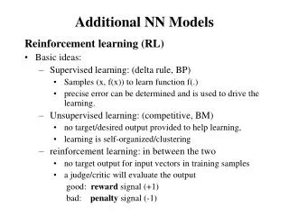
Additional NN Models. Reinforcement learning (RL) Basic ideas: Supervised learning: (delta rule, BP) sample(x, f(s)) to learn f(.) precise error can be determined and is used to drive the learning. Unsupervised learning: (competitive, BM)

Additional NN Models
E N D
Presentation Transcript
Additional NN Models Reinforcement learning (RL) • Basic ideas: • Supervised learning: (delta rule, BP) • sample(x, f(s)) to learn f(.) • precise error can be determined and is used to drive the learning. • Unsupervised learning: (competitive, BM) • no target/desired output provided to help learning, • learning is self-organized/clustering • reinforcement learning: in between the two • no target output for input vectors in training samples • a judge/critic will evaluate the output good: reward signal (+1) bad: penalty signal (-1)
RL exists in many places • Originated from psychology( training animal) • Machine learning community, different theories and algorithms major difficulty: credit/blame distribution chess playing: W/L (multi-step) soccer playing: W/L(multi-player) • In many applications, it is much easier to determine good/bad, right/wrong, acceptable/unacceptable than to provide precise correct answer/error. • It is up to the learning process to improve the system’s performance based on the critic’s signal.
Principle of RL • Let r = +1 reword (good output) r = -1 penalty (bad output) • If r = +1, the system is encouraged to continue what it is doing If r = -1, the system is encouraged not to do what it is doing. • Need to search for better output • because r = -1 does not indicate what the good output should be. • common method is “random search”
critic z(k) y(k) x(k) • ARP: the associative reword-and-penalty algorithm for NN (Barton and Anandan, 1985) • Architecture input: x(k) output: y(k) stochastic units: z(k) for random search
Random search by stochastic units zi or let zi obey a continuous probability distribution function. or let is a random noise, obeys certain distribution. Key: z is not a deterministic function of x, this gives z a chance to be a good output. • Prepare desired output (temporary)
Compute the errors at z layer where E(z(k)) is the expected value of z(k) because z is a random variable How to compute E(z(k)) • take average of z over a period of time • compute from the distribution, if possible • if logistic sigmoid function is used, • Training: BP or other method to minimize the error
(II) Probabilistic Neural Networks 1. Purpose: classify a given input pattern x into one of the pre-defined classes by Bayesian decision rule. Suppose there are k predefined classes s1, …sk P(si): prior probability of class si P(x|si): conditional probability of class si P(x): probability of x P(si|x): posterior probability of si, given x example: S=s1Us2Us3….Usk, the set of all patients si: the set of all patients having disease I x: a description of a patient(manifestation)
P(x|si): prob. One with disease I will have description x P(si|x): prob. one with description x will have disease i. by Bayes’ theorem:
2. PNN architecture: feed forward with 2 hidden layers learning is not used to minimize error but to obtain P(x|si) 3. Learning assumption: P(si) are known, P(x|si) obey Gaussian distr. estimate
4.Comments: (1) Bayesian classification by (2) fast classification( especially if implemented in parallel machine). (3) fast learning (4) trade nodes for time( not good with large training smaples/clusters).
(III)Recurrent BP • Recurrent networks: network with feedback links - state(output) of the network evolves along the time. - may or may not have hidden nodes. - may or may not stabilize when t - how to learn w so that an initial state(input) will lead to a stable state with the desired output. 2. Unfolding for any recurrent network with finite evolution time, there is an equivalent feedforward network. problems: too many repetitions too many layers when the network need a long time to
reach stable state. standard BP needs to be relized to hard duplicate weights. 3. Recurrent BP (1987) system: assume at least one fixed point exists for the system with the given initial state when a fixed point is reduced can be obtained. error
take the gradient descent approach to minimize E by update W direct derivation will have
Computing is very time consuming. Pineda and Almeida/s proposal: can be computed by another recurrent net with identical structure of the original RN direction of each are is reversed( transposed network) in the original network: weight for node j to i: Wij in the transposed network, weight for node j to i:
Weight-update procedure for RBP with a given input and its desired output • Relax the original network to a fixed point • Compute error • Relax the transposed network to a fixed point • Update the weight of the original network
The complete learning algorithm incremental/sequential W is updated by the preseting of each learning pair using the weight-update procedure. to ensure the dearned network is stable, learning rate must be small(much smaller than the rate for standard BP learning) time consuming: two relaxation processes are involved for each step of weight update better performance than BP in some applications
III network of radial basis functions • Motivations better function approximation BP network( hidden units are sigmoid) training time is very long generalization(with non-training input) not always good Counter Propagation(hidden units are WTA) poor approximation, especially with interpolation any input is forced to be classified into one class and intern produces class/ output as its function value.
2. Architecture inputhiddenoutput(similar to BP and CPN) operation/learning: similar to CPN inputhidden: competitive learning for class character hiddenoutput delta rule(LMS error) for mapping difference: hidden units obey Radial Basis function 3. Hidden unit: Gaussian function suppose unit I represent a class of inputs with centroid
Radial basis function input vectors with equal distance to Ci will have the same output. Each hidden unit I has a receptive fied with Ci as its center if x=Ci , unit I has the largest output if x!=Ci, unit I has the smallest output the size of the receptive field is determined by During computation, hidden units are not WTA( no lateral inhibition with an input x, usually more than one hidden units can have non-zero output. These outputs can be combined at output layer to produce better approximation.
4. Learning inputhidden Ci: competitive, based on neti : ad hoc(performance not sensitive to hiddenoutput delta rule(LMS)
5. Comments • compare with BP approximate any …..L2 function(same as BP) may have better … usually requires many more training samples and many more hidden units only one hidden layer is needed. training is faster • Compare with CPN much better function approximation theoretical analysis is only prelimnary

