Computer Network Modeling and Simulation for Performance Analysis
Explore the methodology and tools for modeling and simulating computer networks to analyze performance and evaluate design alternatives. Learn about simulation techniques, model development, and classification of simulation tools.

Computer Network Modeling and Simulation for Performance Analysis
E N D
Presentation Transcript
COMPUTER NETWORK:MODELING AND SIMULATION -Abhaykumar Kumbhar Computer Science Department
Motivation: • Bridge between Real life application and Theoretical world.
Contents: • Introduction. • Modeling. • Simulation. • How to develop a Model. • Classification . • NS simulator. • OPNET. • An Ethernet Case Study. • Requirements of a good Network Simulating Tool • Evolution. • Conclusion and Future Work
Introduction: • Performance analysis of computer networks : increase in size and geographical extent. • The size of the networks and the inherent complexity of network protocols complicate this analysis. • Analysis techniques such as queuing models have difficulty modeling dynamic behavior retransmission timeouts and congestion. • Simulation offers a better method of studying computer networks, since one can simulate the details of actual protocols.
Simulation is an analysis and evaluation tool. • Every simulation is tight to a model that represents the real world. • Inconsistent modeling • Modeling itself is a crucial step towards meaningful results. • Aim :systematic modeling techniques -increase the quality and validity of results
Modeling: • Constructing a conceptual framework that describes a system.
program boundary computer program simulates deterministic rules governing behavior pseudo random inputs to system (models environment) “simulated” life observer Simulation: system boundary system under study (has deterministic rules governing its behavior) exogenous inputs to system (the environment) “real” life observer
Why Simulation? • study system performance, operation • real-system not available, is complex/costly or dangerous (eg: space simulations, flight simulations) • quickly evaluate design alternatives (eg: different system configurations) • evaluate complex functions for which closed form formulas or numerical techniques not available
When to Use Simulation? • Whenever Mathematical Analysis Is Difficult or Impossible. • For Validating Analytic Models. • For Experimentation Without Disturbing an Operational System
How to develop a model: • Determine the goals and objectives • Build a conceptual model • Convert into a specification model • Convert into a computational model • Verify • Validate
Classification of Simulation Tools: • GPPL: General Purpose Programming Language • PSL: “Plain” Simulation Language • SP: Simulation Package
NS Simulator: • Began as REAL in 1989 • Developed by UC Berkeley • Public domain SP • Object-oriented • Written in C++ and object-oriented tcl (Otcl) • Network components are represented by classes
OPNET: • Developed by OPNET Technologies Inc. • Commercial SP • Object-oriented • Totally menu-driven package • Built-in model libraries contain most popular protocols and applications • Simulation task made easy
An Ethernet Case Study: • Bridging the Gap Between Reality and Simulations • We set up our test-bed using two nodes connected by a 3 meter cross-over Ethernet cable. • a simple test-bed experiment and attempt to replicate the obtained results by simulation in ns-2,QualNet and OPNET.
Network details • set packet size of the application to 1472 bytes. This was to ensure that the maximum Ethernet frame of 1500 bytes would be transmitted
Delay experienced by packets in saturated case with non-blocking sockets particularly interested in the saturation performance of the system and we chose multiple rates near the maximum link bandwidth
The maximum delay of the system is experienced when the source bufferis full. • This delay is given as max delay = tx delay ×buffer size in packets. • The transmission delay for one packet is the minimum delay. • The buffer size is then calculated as max delay/min delay. Hence a buffer size of 78 packets was arrived at 94/1.2 ≈ 78packets ≤ 128KB.
Setting up simulations in QualNet: --the link propagation delay being negligible, set it to 25 μs to model test-bed network characteristics. --queue size from its default value of 50 KB to 117 KB, which corresponds to 78 packets of 1500 bytes each.
Setting up simulations in OPNET • Ethernet Station Advanced (ESA). • The ESA has a traffic generator built over the Ethernet MAC. • the queue length to infinity. • OPNET models queues as a set of sub-queues, allowing the possibility of different application traffic to map on to different queues. By default only one sub-queue is created in the Ethernet MAC process model and this is a hidden parameter. This sub queue is accessed as a process interface of the Ethernet MAC process model. The sub-queue packet capacity was set to 78 packets.
Setting up simulations in NS-2 • configurable parameters: node objects, link bandwidth, maximum length and type of the interface queue and delay. • queue length to 78. • maximum propagation delay is 25 μs for 10 Mbps.
Results: • Figure :Throughput
Requirements for Network Simulation tools : • Model development simplicity • Modeling flexibility • Fast modeling • Animation • Different kinds of implemented components • Component adaptability • Creating new components • Static capabilities of a simulator • Graphs
Evolution of Network Simulation Tools: • “Zeroth ” Generation — General Purpose Languages - Fortran, C/C++, Pascal, Basic • “First” Generation — General Purpose Queueing System Simulations -GPSS, SLAM, SIMSCRIPT • “Second” Generation — Application Specific: Computer Systems and Wide-Area Communication Networks • “Third” Generation — Integration of Second Generation Languages -With a Graphics-Oriented Analysis and Modeling Environment -SES/Workbench -OPNET
Conclusion and Future work: • Best way to learn Protocols.
References: 1:Advanced Modelling and Simulation Methods for Communication Networks Jože Mohorko, Fras Matjaž, Klampfer Saša. 2:www.sciencedirect.com 3:www.ieeexplore.org
THANK YOU • QUESTIONS??