Download
1 / 70
710 likes | 1.01k Vues
Chapter 7. Imprint of Climatic Zonation on Marine Sediments. Overall zonation and main factors Biogeographic climate indicators Diversity and shell chemistry as climatic indicators Coral reefs, markers of tropical climate Geological climate indicators

E N D
Chapter 7.Imprint of Climatic Zonation on Marine Sediments • Overall zonation and main factors • Biogeographic climate indicators • Diversity and shell chemistry as climatic indicators • Coral reefs, markers of tropical climate • Geological climate indicators • Climatic clues from restricted seas
7.1 Overall Zonation and Main Factors • The chief factor in producing climatic zonation is the amount of energy received from the sun. • It is high in the tropics, low at the poles. Fig.7.1 a, b. Climatic extremes in the present ocean. a Fringing reef and lagoons, Huahine, Society Islands, tropical South Pacific. [ Courtesy D. L. Eicher] b Tabular iceberg, Antarctic Ocean. [Courtesy T. Foster]
Tropical, subtropical, temperate, and polar, whereby the poleward part of temperate and the more temperate part of polar could be distinguished as subpolar Fig.7.2 Climatic zonation of the open oceans. Zone boundaries tend to follow latitudes and line up with climatic belts on land. Temperature, seasonality, and budget (evaporation-precipitation balance) are the most important descriptors. Approximate temperatures of surface waters in ℃ shown at the boundaries.
Tropical zone • Excess of heat • Seasonal fluctuation are minimal • Average temperatures are near 25°C, with sustained open ocean maxima close to 30°C • Near the Equator, daily rainfall, cloud cover, and weak winds, lead to excess precipitation over evaporation • At the Equator proper fertility is high because of equatorial upwelling • Elsewhere it is low except near continents.
Subtropical zone • The broad region between the tropics proper and the temperature areas • Desert belt, both on land and in the sea • Cloud cover is low, evaporation rates are high and salinities attain values well above average • Annual temperature ranges can be very high • Coastal areas show seasonal upwelling, depending on wind strength.
Temperate zone • Strongly influenced by seasonal change • Rainfall generally exceeds evaporation, and salinities are correspondingly reduced. • Strong temperature gradients, hence strong winds • These force mixing of surface waters with (nutrient-rich) waters in the upper thermocline, along the west-wind drift • The temperate zones are fertile regions. • In the poleward parts of the temperate zones mixing is further enhanced by seasonal breakdown of the thermocline.
Polar areas • Their ice rim fixes the endpoint of the overall temperature gradient, which ultimately controls winds, currents, and evaporation-precipitation patterns. • The climatic zones are not exactly parallel to latitude.
7.1.2 Temperature and Fertility • The most important climatic factors in the ocean, as far as the production and distribution of biogenous sediments. • In the tropics and subtropics, nutrients are limiting to growth. • Here the surface waters become depleted of nutrients because the density gradient hinder upward diffusion of nutrient-rich deep waters. • Surface production is low. • In the coastal zones of the tropics, and in temperate latitude the supply of light and of nutrients both is adequate; here production is high. • Nutrient supply is increased through vertical mixing (upwelling areas): Off California, off Peru, off Africa • Such upwelling is largely seasonal.
Temperature • Temperature imprints itself on sediment patterns. • Directly; ice-generated debris or warm-water coral • Indirectly; through correlations with the productivity Temperature anomalies • Cold anomalies within the subtropics and along the equator • Regions of upwelling • Producers of organic-rich sediments
Temperature and Fertility - Indian Ocean (monsoon climate) • During winter, cold air masses flow off the continent (Northeast monsoon in India) bringing drought and upwelling. • During summer, the circulation is reversed: the Southeast monsoon brings rain from the ocean.
7.2 Biogeographic Climate Indicators • Biogenous sediments are excellent indicators of climate. • Many organisms have narrow ranges of temperature and fertility and the presence of their remains immediately yields excellent clues for climate reconstruction. • Also, the chemistry of the shells can give indication of temperature, salinity, and growth range.
Paleotemperature from transfer methods • The most widespread biogenous deposit on the present sea floor is calcareous ooze. • Foraminifera are climate indicators. • Planktonic forms live in the uppermost 200m of the water column. • About 20 abundant species. • Each climatic zone has one or more characteristic species and a typical abundance pattern of species within it.
Paleotemperature from transfer methods- Some temperature-sensitive species Fig.7.3. Major distributional zonation of planktonic foraminifera. 1 arctic and antarctic; 2 subarctic and subantarctic; 3 transition zone; 4 subtropical; 5 tropical Dominant foraminifera: a; Neogloboquadrinapachyderma, zone 1 left-coiling; b: Globigerinoides, Zone 2; c: Gooborotaliainflata, Zone 3; d: Globorataliatruncatulinoides. Zone 4; e: Globigerinoidesruber, Zones 4 and 5; f: Globigerinoidessacculifer, Zone 5.
7.2.2 Transfer Equations • The agreement between faunal and climatic zonation suggests that it should be possible to reconstruct climate by counting the relative abundance of the species in the sediment assemblages. • Calculating the original surface water temperature by means of transfer equation.
Test = ∑(pi. ti)/pi • Test is a temperature estimate based on an assemblage of foraminifera (or other shells), pi is the proportion of the I-th species and ti its temperature optimum. • The optimum is the temperature at which we find the highest proportion of the species in the calibration set. • The calibration set consists of sea floor surface samples and corresponding surface water temperatures. • For example, we may find that on the sea floor species no. 3 has its highest proportion underneath surface waters with an annual average temperature of 20°C. • We call this its optimum, and designate it as t3.
7.2.3 Application of Transfer Methods: Climatic Transgression Fig.7.4 a, b. Expansion of polar climate in the North Atlantic, 17000 years ago. a Today's sea surface temperature in winter. b Transfer map, winter surface temperature 17000years ago (in ocean), and distribution of ice sheets and pack ice.
The distribution of surface water temperature - and hence of surface currents and water masses - differs greatly for the last ice age maximum (≈17000 years ago) from the present situation. • Today, polar front is just south of Greenland (-2°C isotherm). • During the glacial maximum, the front ran from New York to the Iberian Peninsula. • Norway, and even England, were entirely cut off from the warming influence of the Gulf Stream.
7.2.4 Limitation of the Transfer Model • Exact calibration is difficult: Sediment arriving on the sea floor becomes thoroughly mixed with older sediment. • The problem of differential dissolution: Hence selective preservation of plankton shells on the sea floor.
Fig.7.5 Effect of selective dissolution on the temperature aspect of a mixed coccolith assemblage. Warm-water forms are removed and cold-water species are enriched in the assemblage as dissolution proceeds. 1: Cyclolithellaannula; 2: Cyclococcolithinafragilis; 3 Umbellosphaeratenuis; 4: Duscowphaerathbifera; 5 Emilianiahyxleyi; 6; Umbellosphaerairregularis; 7; Umbilicosphaeramirabilis; 8; Rhabdosphaerastylifera; 9 Helicopontosphaerakamptneri; 10; Cyclococcolithinaleptopora; 11; Gephyrocapsa sp. (includes G. oceanica and G. caribbeanica; the latter is shown); 12: Coccolithuspelagicus. [W. H. Berger, 1973, Deep-Sea Res. 20;917]
Benthic organisms have the same basic requirements as planktonic organisms. • While the remains of plankton on the sea floor are arranged in broad climatic zones, benthic assemblages have a strong regional component. • We refer here to shelf assemblages, as the ones being most affected by climate.
7.3 Diversity and Shell Chemistry as Climatic Indicators 7.3.1 Diversity Gradients • One way to map changing climatic pattern is to focus not on the species themselves but on the statistical patterns they make: their diversity and their dominance. • The number of species is high in the tropics, and low toward the poles. • A diversity gradient, which runs roughly parallel to the global temperature gradient. • In coastal areas, however, anomalously low salinity values or high influx of mud can adversely affect the marine habitat which can lower diversity independently of temperature. • Quite commonly, abundance of certain species are very high in areas of low diversity, because the physical rigor of the environment excludes competition of enemies or both.
7.3.2 Oxygen Isotopes • Relationship between shell chemistry and environment • Carbonates precipitated from the same aqueous solution should have different 18O/16O, depending on the temperature at which the precipitation proceeds. • Paleotemperature determination: • t = 16.5 - 4.3 (s - w) + (s - w)2 • t is the temperature, • δs is the oxygen isotope composition of the shell sample, • δw is that of the water the shell grew in. • 18O, expressed in per mil • Isotopic equilibrium • Salinity effect
7.3.3 Carbon Isotopes (13C/12C) • These also have a temperature dependence, but less • The main effect on their ratio appears to be the metabolic activity of the shell-secreting organisms. • Source of carbon
7.3.4 Other Chemical Markers • Magnesium in calcareous shells tends to increase with temperature. • Sr and other trace elements • This effect appears to be more pronounced in the lower organisms such as calcareous algae and foraminifera, than in the higher ones, for example the barnacles.
7.4 Coral Reefs, Markers of Tropical Climate • The reef association indicates tropical shallow waters. • Reefs extend into the subtropics on the western sides of the ocean basins, and are greatly restricted on the eastern sides. • The warm western and eastern boundary currents are responsible for carrying the reef limits to their latitudinal extremes. Fig.7.6 Distribution of coral reefs (hachured areas). 20℃ isotherm for coldest month of the year shown as heavy line. Note the general correspondence. Areas of coastal upwelling (triangles) inhibit coral growth. Hence the eastern margins are unfavorable for reef development. Present maximum equatorward extent of iceberg drift also is shown.
7.4.2 Reef building • Up to 10,000 g/m2 of CaCO3 can be produced annually, with a rate of upbuilding of 10 mm/yr • Calcareous ooze; accumulation rate near 10 g/m2/yr. • About 50% of the reef is solid matter and 50% is empty space. • Where the sea floor sinks, reefs can build enormous shelf bodies (on continental margins), or mountain peaks (on sunken volcanoes). 1) framework (the supporting structure); corals, calcareous algae 2) fill; the fill between the framework consists of reef debris and the hard parts of various other reef inhabitants.
The reef offers an extraordinary variety of life styles Solid substrate favors eqibionts such as bryozoans and sessile foraminifera Cavities offer shelter for fishes and crustaceans. Fig.7.7 Stone coral colony with associated macrofauna, classified as to mode of feeding. The dead basal part of the coral forms a hard substrate on which epibenthos settles. Note the boring organisms (e. g., cliona) which gelp destroy coral structures. [S. Gerlach, 1959, verh Dtsch Zool Ges 356]
The tropical reef • Greatest diversity: More than 3,000 species live in Indo-Pacific reefs. • The skeletal remains produced in rich variety are broken up in various ways, by boring algae, sponges and sea urchins and crushed by fishes and crustaceans; Production of carbonate sand. • In many skeletons, calcite crystals are held together by organic material. • When it decays such skeletons disintegrate to lime mud; Production of carbonate mud.
7.4.3 Atolls • Charles Darwin first explained their origin • A sequence going from fringing reef to barrier reef to atoll (Subsidence theory). • Since the algae, both as carbonate producers and as symbionts of corals, need light, the coral reefs can only grow in very shallow water. • An atoll, therefore, cannot have grown up from deep waters. • This is the reasoning that led Darwin to propose a combination of slowly sinking sea floor and upbuilding of reef. Fig.7.8 Darwin's hypothesis of atoll formation. Redrawn, with maps by Darwin (right) to show the resemblance in form between barrier coral reefs surrounding mountainous islands, and atolls of lagoon islands. [C. Darwin, 1842. On the structure and distribution of coral reefs, Ward Lock & Co. London]
7.5 Geologic Climate Indicators 7.5.1 Chemical indicators Fig.7.9 Distribution of shelf deposits in relation to climatic zonation, in the northern half of an idealized ocean basin. Continents black. Current shown as arrows. Detrital refers to terrigenous river influx, authigenic to phosphatic deposits associated with organic-rich sediments, biogenic to carbonates (mollusks, foraminifera, corals, and algae). Shell carbonate is produced outside the tropics as well but tends to be masked by terrigenous supply. Restricted shelf seas collect carbon-rich (C) or evaporitic sediment (E) depending on climate zone.
Simple compilation of reef occurrences through time indicate the position of the equatorial belt and, ultimately, the cross-latitudinal motion of the continent. • Biogenous carbonate deposits in general quite similar clues. • Salt and dolomite deposits also have been used to delineate climatic belts. • They are characteristic for the subtropics and result from excess evaporation. • In tropical areas, laterite and the clay mineral kaolinite are typical weathering products.
7.5.2 Physical Geologic indicators • Physical geologic indicators are especially obvious in high latitudes, due to the effect of ice. • On shelves entirely covered by ice, as in the Antarctic, erosion predominates. • Bare rock, polished and scratched, dominates; morainal debris fills depressions. • Iceberg calving from glaciers take enclosed debris with them, and release it on melting. • End moraines in their typical lobe-shaped morphology.
Sea Ice Fig.7.10 Ice-sheet depositional model. [A. K. Cooper et al. 1001, Marine Geol 102, 180]
The sea ice, 1 to 4 m thick, hinders the transport of sediment by dampening waves and longshore currents. • The absence of sufficient longshore transport can perhaps explain the scarcity of lagoons in the Arctic. • The sea ice also shields the entire Arctic sea floor from pelagic sediment supply: sedimentation rates in the central Arctic ocean are extraordinarily low (≈1 mm/1000 years) • Arctic environments are very demanding, as regards benthic life. • Paucity of species is characteristic; WHY?
WHY? • On freezing, salt is largely excluded from the ice; thus the salinity of the remaining water is increased to more than 65 %. • When the ice and the snow cover melts, in early summer, the water is diluted to a salinity of 2 ‰. • When the sea ice melts, in mid-summer, normal marine waters enter the lagoon and salinity increases to 30 ‰. • In October, the lagoon freezes over again, the cycle starts anew. • Clearly, only a very few types of shell-producing organisms (or burrowers) can be expected under such extreme conditions.
Particle Size • The supply from rivers in high latitudes appears to consist mainly of silt, with clay and sand being distinctly subordinate. • This is an interesting sedimentologic phenomenon, presumably it is caused by mechanical weathering through the freeze-thaw cycle. • The process is important in producing loess, the silty sediment blown out from glaciated area and piled up in their perimeter.
7.6 Climatic Clues from Restricted Seas 7.6.1 Salinity distributions and exchange patterns • Arid and humid; the balance between evaporation and precipitation. • Climate-produced salinity differences in the open ocean are present, and outline the major patterns of evaporation excess (central gyres) and precipitation excess (equator, temperate to high latitudes) Fig.7.11 a, b. Evaporation/precipitation patterns in the world ocean, and corresponding salinity distribution. a Map showing difference between precipitation and evaporation. b Surface water salinities of the ocean, averaged by latitude, and compared with evaporation-minus-precipitation values.
The salinity differences in the open sea are too small to leave much of a direct record via inorganic or biogenous sedimentation. • However, the differences are amplified in the restricted seas adjacent to the ocean basins.
Two types of circulation; profound consequence for its fertility and sedimentation Fig.7.12 Anti-estuarine and estuarine circulation in basins with excess evaporation and with excess precipitation, respectively, The arid basin (A) is characterized by downwelling, hence low fertility and high oxygen content. The estuarine basin (B) is characterized by upwelling and salinity stratification, hence high fertility and low oxygen content. The geographic names above the graph give three examples each for anti-estuarine and estuarine circulation
Anti-estuarine circulation • The seas in the arid belt, with excess evaporation, have a common typical exchange pattern with the open ocean: shallow-in, deep-out • the Mediterranean, the Persian Gulf, and the Red Sea • downwelling, hence low fertility and high oxygen content
Estuarine circulation • Where rain and river influx exceeds evaporation, sea level rises, and the water in the humid sea is freshened out and becomes lighter than open ocean water. • Thus, the heavier ocean water pushes in at depth and displaces the less saline water from below. • The incoming water is subsurface water; deep-in, and shallow-out. • the Black Sea, the Baltic, and the fjords of Alaska and Norway. • upwelling and salinity stratification, hence high fertility and low oxygen content
7.6.2 The Baltic as humid model of a marginal sea – Estuarine! • In the Baltic, the fully marine fauna off the entrance is gradually reduced in going deeper into the basin. • Correspondingly, the dominance of certain brackish-tolerant species greatly increases. • The marine mulluscs become smaller and their shells thinner. Table 7.1 Decrease of species from open ocean into Baltic.(After Remane 1958)
Baltic Sea • Easily freshen out, depending on precipitation, influx, and degree of isolation. • In such enclosed embayments, reeds and other plants grow to build up peat, eventually to be fossilized to coaly layers. • Finally, stratification of the water column is much more stable in the Baltic than in the Persian Gulf, due to the high density contrast between brackish surface water and saline deep water. • Without vertical mixing, no new oxygen can be supplied to the deep waters from the surface waters which are in contact with the atmosphere.
Baltic Sea • Productivity in the Baltic sea is high because nutrient-rich subsurface waters enter from the North Sea. • The high supply of nutrients within the basin leads to high productivity which in turn delivers much organic matter to the sea floor. • Oxygen is rapidly used up by the decay of this matter. • Especially during periods of stable stratification, the bottom water develops a serious oxygen deficiency, with values of less than 10% of saturation. • Under certain conditions all the oxygen can be used up, and H2S develops from bacterial sulfate reduction.
Fig.7.13 Bathymetric distribution of the abundant benthic foraminifera in the western Baltic. Width of black columns indicates number of living specimens found per 10㎠ seabottom (Ammoscalaria; only empty shells were found in 1963/63). The wavy line at about 14m depth marks the boundary between outflowing surface water and incoming marine water.
7.6.3 Conditions of stagnation • At a concentration of less than 1 ml O2 per liter of water, shelled organisms disappear. • Only a few species of metazoans remain: mainly worms (annelids, nematodes) and crustaceans. • Below 0.1 ml O2 per liter the environment becomes hostile to all metazoans; only some protists and anaerobic bacteria survive.
Conditions of stagnation 2 • As mentioned, both high productivity and stable stratification are responsible for the oxygen deficiency in Baltic bottom waters. • Finely laminated sediments, with layers of millimeter dimensions: These layers indicate the absence of deposit feeders and other burrowers, hence they show the absence of oxygen.
Conditions of stagnation 3 • The chemistry of anaerobic sediments is complex. • The CO2 concentration in the bottom-near water with very low O2 content is high: CO2 is produced as the O2 is used up. • CO2 and water produce carbonic acid, and the pH drops (to less than 7, compared with open ocean values near 8). • Consequently, calcareous shells are dissolved on the sea floor. • High CO2 content of interstitial waters also means that hydrogenous carbonates can form.
Conditions of stagnation 4 • Manganese is readily mobilized under conditions of oxygen deficiency, migrates upward in the sediment as Mn2+. • It is kept on the sea floor both by oxidation and precipitation as oxide (MnO2) and as manganese carbonate (MnCO3) which forms under conditions of anaerobism and high CO2 concentrations. • Iron carbonate also may form, although iron is less mobile, being readily precipitated both as sulfide and as oxide.
Conditions of stagnation 5 • When free oxygen is gone, bacteria produce sulfide by the reduction of sulfate ion • SO42- + 2CH2O → H2S +2HCO3- • Iron sulfide forms under these conditions; hence pyrite crystals (FeS2) are common in black anaerobic sediments. • If sulfate reduction occurs at the very surface of the sediment, calcareous shells are preserved.