ENGINEERING ECONOMICS
ENGINEERING ECONOMICS. Lecture # 3 Cash Flow and Cash Flow Diagram Rule of 72 Arithmetic Gradient Factor Geometric Gradient Factor Total present worth Examples and Numerical. Cash Flow.

ENGINEERING ECONOMICS
E N D
Presentation Transcript
ENGINEERING ECONOMICS Lecture # 3 Cash Flow and Cash Flow Diagram Rule of 72 Arithmetic Gradient Factor Geometric Gradient Factor Total present worth Examples and Numerical
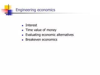
Cash Flow • Engineering projects generally have economic consequences that occur over an extended period of time • Each project is described as cash receipts or disbursements (expenses) at different points in time • For any practical engineering economy problems, the cash flows must be:- • Known with certainty • Estimated • Range of possible realistic values • Generated from assumed distribution and simulation
Categories of Cash Flows • The expenses and receipts due to engineering projects usually fall into one of the following categories: • First cost: expense to build or to buy and install • Operations and maintenance (O&M): annual expense, such as electricity, labor, and minor repairs • Salvage value: receipt at project termination for sale or transfer of the equipment (can be a salvage cost) • Revenues: annual receipts due to sale of products or services • Overhaul: major capital expenditure that occurs during the asset’s life
Cash Flow Diagrams • The costs and benefits of engineering projects over time are summarized on a cash flow diagram (CFD). Specifically, CFD illustrates the size, sign, and timing of individual cash flows, and forms the basis for engineering economic analysis • A CFD is created by first drawing a segmented time-based horizontal line, divided into appropriate time unit. Each time when there is a cash flow, a vertical arrow is added pointing down for costs and up for revenues or benefits. The cost flows are drawn to relative scale
An Example of Cash Flow Diagram • A man borrowed $1,000 from a bank at 8% interest. Two end-of-year payments: at the end of the first year, he will repay half of the $1000 principal plus the interest that is due. At the end of the second year, he will repay the remaining half plus the interest for the second year. • Cash flow for this problem is: End of year Cash flow 0 +$1000 1 -$580 (-$500 - $80) 2 -$540 (-$500 - $40)
$1,000 1 2 0 $540 $580 Cash Flow Diagram
Important Aspects of CFD • Extremely valuable analysis tool • First step in solution process • Graphical representation on a time scale • Does not have to be drawn to exact scale • Information in one glance
Cash Flow Diagram • Used to describe any investment opportunity. • Inflow (revenue) • Outflow (costs) 0 Make an initial investment (purchase) at “time 0” P
Cash Flow Diagram The net amount is written on the cash flow diagram 0 1 2 T Receive revenues and pay expenses over time. P
Cash Flow Diagram 0 1 2 T Write as a NET cash flow in each period. P
Cash Flow Diagram SV 0 1 2 T Receive salvage value at end of life of project. P
Time Value of Money Generally, money grows (compounds) into larger future sums and is smaller (discounted ) in the past
Compound Interest and Cash Flow Diagrams • Example: P=$1000, i=10%, compounded annually. • How much accrued after two years? F = 1210 0 1 2 P = 1000 In general: F = P(1+i)n
Steps to Solve Time Value of Money Problems 1. Read problem thoroughly 2. Create a time line 3. Put cash flows and arrows on time line 4. Determine if it is a PV or FV problem • Determine if solution involves annuity • Solve the problem
Rule of 72 • Investors most often ask • How long will it take for my investment to be doubled in the value? • Can I have a known or assumed compound interest rate in advance?
Rule of 72 • The approximate time for an investment to be doubled in value given the compound interest rate is • n = 72 / i • For example if i = 13% then time = 72 / 13 = 5.54 years
Rule of 72 • One can estimate the future required interest rate for an investment to be doubled in value over time • i = 72 / n • Assume that we want the investment to be doubled in 3 years • i = 72 / 3 = 24%
Arithmetic Gradient • It is a cash flow series that either increases or decreases by constant amount • The cash flow changes by the same arithmetic amount each period • The amount of increase or decrease is the gradient • If it is predicted that the cost of NOKIA mobile will increase by Rs 2000 each year, a gradient series is involved and the amount of gradient is Rs 2000 • G = Constant arithmetic change (+ or -)
Arithmetic Gradient - Formulae • i = annual interest rate • n = interest period • P = present principle amount • A = Equal annual payments • F = Future amount • G = Annual change or gradient
Factors • F / P = Single payment future worth factor • P / F = Single payment present worth factor • F / A = Equal payment series future worth factor • A / F = Equal payment series sinking fund factor • P / A = Equal payment series present worth factor • A / P = Equal payment series capital recovery factor • A / G = Arithmetic gradient series factor • F / G = Arithmetic gradient future worth factor • P / G = Arithmetic gradient present worth factor • Geometric Gradient factor (only definition)
Total Present Worth in Gradient Problems (Pt) • The total present worth of a gradient series must consider the base and the gradient separately • The base amount is the uniform series amount that begins in year 1 and extends through year n. It is represented by P1 • For an increasing gradient, the gradient amount must be added to the uniform series amount. It is represented by P2 • For a decreasing gradient, the gradient amount must be subtracted from the uniform series amount. It is represented by –P2 • Pt = P1 + P2 • Pt = P1 – P2
F / P = Single payment future worth factor F = P (1 + i)n F / P = (1 + i)n P / F = Single payment present worth factor 1 / (1 + i)n = P/F
F / A = Equal payment series future worth factor What will be the future worth of an amount of $ 100 deposited at the end of each next five years and earning 12 % per annum? A / F = Equal payment series sinking fund factor It is desired to accumulate $ 635 by making a series of five equal annual payments at 12 % interest annually, what will be the required amount of each payment?
A / P = Equal payment series capital recovery factor A car has useful life of 5 years. The maintenance cost occurs at the end of each year. The owner wants to set up an account which earns 12 % annually on an amount of $ 3604 to cater for this maintenance cost. What is the maintenance cost per annum?
Geometric Gradient • It is common for cash flow series such as operating cost, construction cost and revenues to increase or decrease by a constant percentage such as 10 % • This uniform rate of change in %age is called geometric gradient = g • g = constant rate of change in %age or decimal form by which amount increase or decreases from one period to other