Download
1 / 33
460 likes | 1.11k Vues
Growth Curve Models Using Multilevel Modeling with SPSS. David A. Kenny. Presumed Background. Multilevel Modeling Nested. Basic Idea. Used to examine linear and nonlinear changes over time Time the key predictor variable in growth models Need at least three time points to model growth.

E N D
Growth Curve Models Using Multilevel Modeling with SPSS David A. Kenny
Presumed Background • Multilevel Modeling • Nested
Basic Idea • Used to examine linear and nonlinear changes over time • Time the key predictor variable in growth models • Need at least three time points to model growth
Multilevel Model • Levels • Level 1: Times • Level 2: Persons • Spacing of time points • Each individual need not have the same number of time points • Difference between time points need be the same • Time points can be different for each person
Data Structure A person period dataset Each record is one time for each person Sometimes called a “narrow” format as opposed to a “wide” format which has all the person’s times on one record.
Example Data Campbell, L., Simpson, J. A., Boldry, J. G., & Kashy, D. A. (2005). Perceptions of Conflict and Support in Romantic Relationships: The Role of Attachment Anxiety. Journal of Personality and Social Psychology, 88, 510-531. 103 Dating Couples completing a 14-day daily diary study Consider only the males
Download • Data • Syntax • Output
Variables • satisf: Satisfaction with the Relationship, measured on a 1 to 7 scale • day: Day of survey from 1 to 14 • time: measured in weeks and centered; equals (day – 7.5)/7 • avoidc: attachment avoidance centered (grand mean across both men and women subtracted) • Missing cases • One person and his partner is missing the Attachment measure • There are 11 missing satisfaction scores. • Total number of cases: 103 x 14 – 25 = 1417
Defining Time Zero for Growth Models • The intercept refers to the predicted score when time equals zero. • Thus, the scaling of time affects the intercept’s meaning. • Some common options for modeling the intercept • Initial measurement (the usual option) • Study midpoint • Time of intervention • Study endpoint • In the Kashy data set, 7.5 is subtracted off of each time since there are 14 time points 11
Fixed Effect Equation satisfaction = intercept + b(time) + c(avoidc) + d(time*avoidc) + error Intercept = predicted satisfaction score at the study midpoint (when time = 0) b = the predicted change in satisfaction as time for a week If the main effect of time is positive then satisfaction is increasing over time and if it is negative then satisfaction is decreasing. c = effect of avoidance attachment on satisfaction d = Does the effect of time on satisfaction change as a function of avoidance attachment? Error = the part of satisfaction that is not predicted by time and avoidant attachment.
Random Effects Variance of the intercepts • based on the variance of how much men vary in satisfaction at study midpoint Variance of the slopes • How much men vary in their rate of linear change in satisfaction Covariance between the intercept and slope • Do individuals who have higher satisfaction scores at the study midpoint change more rapidly (or slowly) than those with lower satisfaction scores at midpoint?
SPSS Syntax MIXED satisf WITH time avoidc /FIXED=time avoidc time*avoidc /PRINT=SOLUTION TESTCOV /RANDOM=INTERCEPT time | SUBJECT(personid) COVTYPE(UNR). “RANDOM INTERCEPT time” Estimates a random intercept and slope variance. UNR provides a correlation between slope and intercept.
Satisfaction = 6.26 + 0.134(Time) + -0.140(Avoid) + 0.032(Time*Avoid) • Intercept = 6.26 • The average level of satisfaction at time = 0 • Coefficient for Time = 0.134 • Over time, satisfaction increases .134 units a week • The slope is small, although it is statistically significant. There is some evidence of an average increase in satisfaction over time for men. • Coefficient for Avoidance = -0.140 • More Avoidance less satisfaction • No interaction of Time and Avoidance
SPSS Output Random Effects Random Effects Variance of Intercepts: Var(1) = .460* Variance of Slopes: Var(2) = .124* Correlation Inter./Slope: Corr(2,1) = -.032 /RANDOM INTERCEPT time | SUBJECT(personid) COVTYPE(UNR). With SPSS, p values for variances (not correlations) must be divided by two to make the p values one-sided.
Random Effects • Random effects: • Variance in the intercepts • some men were more satisfied than others at the midpoint. • Variance in the slopes • some men are changing in satisfaction more than others. • Slope-intercept covariance • Men with higher values at time 0 change more slowly than those with lower values, but this correlation is not significant and small.
Autoregressive Errors • Bolger, N., & Laurenceau, J.-P. (2013). Intensive longitudinal methods: An introduction to diary and experience sampling research. New York: Guilford Press. • They suggest having errors that affect one another: e1 e2 e3 autoregressive errors
SPSS Syntax MIXED satisf WITH time avoidc /FIXED=time avoidc time*avoidc /PRINT=SOLUTION TESTCOV /RANDOM=INTERCEPT time | SUBJECT(personid) COVTYPE(UNR) /REPEATED day | SUBJECT(personid) COVTYPE(AR1).
Changes Half as much slope variance
Convergence Issues: SPSS • Sometimes run will not converge and you get the message: • What to do? • Theoretical Solutions • Computational Solutions
Theoretical • Possibilities • A variance component you want to estimate is very small. • Two variance components are too highly correlated. • Solution: Drop or combine component. • Note if a variance component is estimated as zero, you always get this warning.
Computational • SPSS is poor at finding a solution: Use another program. • SPSS changes • Change UNR to UN. • If a predictor is random (e.g., time) increase the size of its variance by decreasing the variance of a predictor. • That was why the units for “time” is weeks not “days.” • Make the following changes on the “Estimation” screen:
Increase These are things that work for me. There may well be better options. Increase Increase
Thanks! Debby Kashy Tessa West
More Webinars References (pdf) Programs Repeated Measures Two-Intercept Model Crossed Design Other Topics