Linear Programming Application for Production Planning in Semiconductor Manufacturing
340 likes | 625 Vues
Linear Programming Application for Production Planning in Semiconductor Manufacturing. 공장자동화연구실 이기창 1998/04/07. Introduction(1/3). Semiconductor manufacturing processes. Introduction(2/3). Characteristics of semiconductor manufacturing Complexities Cyclic processes

Linear Programming Application for Production Planning in Semiconductor Manufacturing
E N D
Presentation Transcript
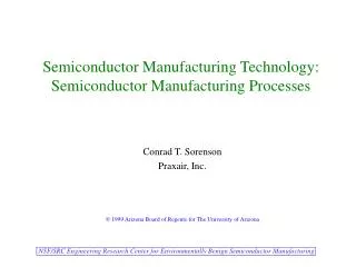
Linear Programming Application for Production Planning in Semiconductor Manufacturing 공장자동화연구실 이기창 1998/04/07
Introduction(1/3) • Semiconductor manufacturing processes
Introduction(2/3) • Characteristics of semiconductor manufacturing • Complexities • Cyclic processes • Several different recipes • Uncertain yields • Characteristics of production planning • Variable flow time • Time-consuming production planning
Introduction(3/3) • Favored objective function • Demand satisfaction • Maximum utilization • Maximum throughput • Terminology • Wafer fab : front-end manufacturing facility • Wafer : individual unit of processing material • Die : integrated circuit
Research overview • Golovin(1986) - integrated mathematical formulation • Leachman(1992) - general modeling framework • Uzsoy(1992) - a review • Katayama(1996) - variable yield rate evaluation • Lee(1997) - variable cycle time
A Production Planning Methodology for Semiconductor Manufacturing based on Iterative Simulation and Linear Programming Calculations Yi-Feng Hung and Robert C.Leachman Dep. Of Industrial Engineering, National Tsing Hua University, Taiwan. Engineering Systems Research Center, University of California at Berceley, USA. IEEE Transactions on semiconductor manufacturing, Vol.9, No.2, 1996
Assumptions of LP formulation • Demands, capacities and production rates in a planning period are constant. • Release quantity in a period is to be distributed uniformly over the period. • Production variable is quantity of a wafer type to be released in a period. • Inventory variable is inventory level of a wafer type at the end of a period. • Backorders are allowed with costs. • Workload includes machine hours due to WIP and planned releases.
Basic LP formulation • Max • die output revenue - raw material cost - die inventory holding cost - cost of backordered die demands • Subject to • m/c hours for new releases <= available m/c hours - m/c hours for WIP • die output during the period + inventory at the start of period - backorders at the start of period - inventory at the end of period + backorders at the end of period = demands during the period
Notation : # of working days on route i from start of period 1 until the end of period p : smallest index p such that : the expected flow time from wafer release to operation l occurring at epoch of route i : the expected flow time from wafer release to finish occurring at epoch of route i : wafer release quantity for route i in period p : wafer quantity consuming M/C hours at operation l of route i in period p : wafer quantity from route i in period p
Loads representation in terms of release variables (2/2) Case (1) Case (2)
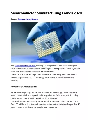
Simulation model • Test data set • Micron Technology • 10 types of products(wafers) • 2 types of demands (customer order and potential sales) • Each route has 86~187operations including 30 workstations • Assumption • Each workstation have MTBF and MTTR parameters. • All operations are lot-based(size 50 wafers).
Iterative scheme • Approach • To embed flow times predicted by simulation in an LP model • To convert wafer release of LP to discrete lots of simulation model • To run a simulation model using the release schedule from the LP • To collect statistics on flow time during simulation run
Computational experiments (1/6) • Deterministic simulation model
Computational experiments (4/6) • Simulation model with machine failures
Conclusion • Iterative planning calculation generates accurate production plan. • Calculation time is applicable to real shop. • 2 hours for one iteration • 7 iterations is enough to get acceptable flow time agreement • Analytical model instead of simulation model could be developed. • Alternative machine types are to be included.
A New Formulation Technique for Alternative Material Planning - An Approach for Semiconductor Bin Allocation Planning Y.F.Hung and Q.Z.Wang Dep. Of Industrial Engineering, National Tsing Hua University, Taiwan, ROC. Computers and Industrial Engineering, Vol.32, No.2, 1997.
Alternative material planning • Formulating as transportation problem
Alternative material planning • Formulating as transshipment problem
Conventional bin allocation allocation planning formulation(1/2)
Conventional bin allocation allocation planning formulation(2/2) Objective function (1) Bin inventory balance (2) Allocation constraint (3) Demand constraint
New formulation for bin allocation planning(2/2) (1) Acceptable bin constraint (2) Demand constraint
Acceptable material set generation procedure • Step1 • Determine the set of supply nodes for each demand node. • Step2 • Whenever Sk1=Sk2 and k1k2, Dk1=Dk1 Dk2 • Step3 • Whenever there exists a s such that s in Sk1, s in Sk2 Sk1USk2 is new supply set, Sk=Sk1 Sk2, Dk=Dk1 Dk2 • Step4 • Whenever Sk1 Sk2, Dk1=Dk1Dk2
Saving of new formulation over the conventional one Straight downbinning case Number of constraints Number of variables Conventional formulation 3M M(M+1)/2+2M New formulation 3M-1 2M Non-straight downbinning case Number of constraints Number of variables Conventional formulation M+2N 2M+N< < M+N+MN New formulation N+M< <2^M -1 M+N
Conclusion • New formulation technique for alternative material planning problem is presented. • Network for all periods is decomposed to separate independent network for each period. • New technique needs 2/3 of the rows of formulation by conventional technique. • Detailed production plan is generated each period incorporating update WIP and demand data.