Conic Sections
Chapter 10. Conic Sections. The Parabola and the Circle. § 10.1. Conic Sections. Parabola. Ellipse. Circle. Hyperbola. Conic sections derive their name because each conic section is the intersection of a right circular cone and a plane. The Parabola. y. y. y. y. x. x. x. x.

Conic Sections
E N D
Presentation Transcript
Chapter 10 Conic Sections
The Parabola and the Circle § 10.1
Conic Sections Parabola Ellipse Circle Hyperbola Conic sections derive their name because each conic section is the intersection of a right circular cone and a plane.
The Parabola y y y y x x x x Just as y = a(x – h)2 + k is the equation of a parabola that opens upward or downward, x = a(y – k)2 + h is the equation of a parabola that opens to the right or to the left. y = a(x – h)2 + k x = a(y – k)2 + h a > 0 (h, k) (h, k) (h, k) y = k a < 0 y = k (h, k) a < 0 a > 0 x = h x = h
The Parabola Example: Graph the parabola x = (y – 4)2 + 1. • a > 0, so the parabola opens to the right. • The vertex of the parabola is (1, 4). • The axis of symmetry is y = 4.
y 2 x 2 The Parabola Example continued: The table shows ordered pairs of the solutions of x = (y – 4)2 + 1. 1 4 y = 4 2 3 2 5 17 0 17 8
The Parabola Example: Graph the parabola y = x2 + 12x + 25. • Complete the square on x to write the equation in standard form. y – 25 = x2 + 12x Subtract 25 from both sides. • The coefficient of x is 12. The square of half of 12 is 62 = 36. y – 25 + 36 = x2 + 12x + 36 Add 36 to both sides.
The Parabola Example continued: y + 11 = (x + 6)2 Simplify the left side and factor the right side. y = (x + 6)2 – 11 Subtract 11 from both sides. • a > 0, so the parabola opens upward. • The vertex of the parabola is (– 6, – 11). • The axis of symmetry is x = – 6.
y 3 x 3 The Parabola Example continued: y = x2 + 12x + 25
Distance Formula The distance d between any two points (x1, y1) and (x2, y2) is given by y (x2, y2) d b = y2 – y1 x (x1, y1) a = x2 – x1 The Distance Formula
The Distance Formula Example: Find the distance between (– 6, – 6) and (– 5, – 2).
Midpoint Formula The midpoint of the line segment whose endpoints are (x1, y1) and (x2, y2) is the point with the coordinates The Midpoint • The midpoint of a line segment is the point located exactly halfway between the two endpoints of the line segment.
The Midpoint Example: Find the midpoint of the line segment that joins points P(0, 8) and Q(4, – 6).
y r (h, k) x The Cirlce A circle is the set of all points in a plane that are the same distance from a fixed point called the center. The distance is called the radius. Circle The graph of (x – h)2 + (y – k)2 = r2 is a circle with center (h, k) and radius r.
y r = 3 x (3, 0) The Circle Example: Graph (x – 3)2 + y2 = 9. The equation can be written as (x– 3)2 + (y– 0)2 = 32. h = 3, k = 0, and r = 3.
The Circle Example: Find the equation of the circle with center (– 7, 6) and radius 2. • h = – 7, k = 6, and r = 2. • (x – h)2 + (y – k)2 = r2. The equation can be written as [x – (– 7)2] + (y – 6)2 = 22. Simplify. (x + 7)2 + (y – 6)2 = 4.
§ 10.2 The Ellipse and the Hyperbola
An ellipse can be thought of as the set of points in a plane such that the sum of the distances of those points from two fixed points is constant. Each of the two fixed points is called a focus. (The plural of focus is foci.) The point midway between the foci is called the center. The Ellipse
Ellipse with Center (0, 0) The graph of an equation of the form is an ellipse with center (0, 0). The x-intercepts are (a, 0) and (– a, 0), and the y-intercepts are (0, b) and (0, – b). y b – a a x – b The Ellipse
y 3 x – 2 2 – 3 The Ellipse Example: • The equation is of the form • a = 2 and b = 3.
An hyperbola can be thought of as the set of points in a plane such that the absolute value of the difference of the distances of those points from two fixed points is constant. Each of the two fixed points is called a focus. (The plural of focus is foci.) The point midway between the foci is called the center. The Hyperbola
The graph of an equation of the form is a hyperbola with center (0, 0) and y-intercepts (0, b) and (0, – b). y x a a y b x The graph of an equation of the form is a hyperbola with center (0, 0) and x-intercepts (a, 0) and (– a, 0). b The Hyperbola Hyperbola with Center (0, 0)
The asymptotes of the hyperbola are dashed lines used to sketch the graph of the hyperbola. To sketch the asymptotes, draw a rectangle with vertices (a, b), (– a, b), (a, – b), and (– a, – b). y b ( a, b) (a, b) x a a (a, b) ( a, b) b Asymptotes
The equation is of the form so its graph is a hyperbola that opens to the left and right. The Hyperbola Example: • It has center (0, 0) and x-intercepts (3, 0) and (– 3, 0). • The asymptotes of the hyperbola are the extended diagonals of the rectangle with corners (3, 6), (– 3, 6), (3, – 6), and (– 3, – 6 ).
y ( 3, 6) (3, 6) 2 x – 2 2 – 2 ( 3, 6) (3, 6) The Hyperbola Example continued:
§ 10.3 Solving Nonlinear Systems of Equations
A nonlinear system of equations is a system of equations where at least one of the equations is not linear. The substitution method or the elimination method may be used to solve the system. Nonlinear Systems of Equations
Nonlinear Systems of Equations Example: Solve the system. The substitution method will work best to solve this system. y + 2 = x Second equation x2 + y = 4 First equation (y + 2)2 + y = 4 Replace x with y + 2. y2 + 4y + 4 + y = 4
Nonlinear Systems of Equations Example continued: y2 + 4y + 4 + y = 4 y2 + 5y = 0 y(y + 5) = 0 y = 0 or y = – 5 Let y = 0 and then let y = – 5 to find the corresponding x values. Let y = 0 Let y = – 5 y+ 2 = x y + 2 = x 0 + 2 = x – 5 + 2 = x x = 2 x = – 3
Nonlinear Systems of Equations y x Example continued: The solutions are (2, 0) and (– 3, – 5). Check both solutions in both equations. x2 + y = 4 y + 2 = x x2 + y = 4 y + 2 = x (– 3)2+ (– 5) = 4 – 5 + 2 = – 3 22 + 0 = 4 0 + 2 = 2 9 – 5 = 4 – 3= – 3 4 = 4 2 = 2 y + 2 = x x2 + y = 4 A graph of the system also verifies the solution. (2, 0) (– 3, – 5).
Nonlinear Systems of Equations Example: Solve the system. The elimination method will work best to solve this system. (– 1) x2 + (– 1) 2y2 = (– 1) 4 Multiply the first equation by – 1. – x2 + – 2y2 = – 4 x2 – y2 = 4 – 3y2 = 0 Add the two equations.
Nonlinear Systems of Equations Example continued: – 3y2 = 0 y = 0 Let y = 0 to find the corresponding x values. x2 + 2y2 = 4 x2 + 2(0)2 = 4 x2 = 4 x = 2 or x = – 2 The solutions are (– 2, 0) and (2, 0). Check both solutions in both equations.
§ 10.4 Nonlinear Inequalities and Systems of Inequalities
Nonlinear inequalities in two variables are graphed in a similar way to linear inequalities in two variables. Nonlinear Inequalities
Nonlinear Inequalities Graph the equation 3 – 4 4 y – 3 Sketch a dashed curve since the graph of does not include the graph of x Example:
Nonlinear Inequalities 3 (0, 0) – 4 4 – 3 y x Example continued: Select a test point to determine which region contains the solutions. Select the test point (0, 0) if it is not on the boundary line. This is a true statement, so the test point is part of the solution.
Nonlinear Inequalities Graph the equation 2 – 2 2 – 2 y Sketch a solid curve since the graph of does include the graph of x Example:
Nonlinear Inequalities (0, 4) (0, 0) 2 – 2 2 – 2 (0, – 4 ) y x Region A Example continued: The hyperbola divides the plane into three regions. Select a test point in each region to determine the solutions. Region B Region A Region B Region C Region C False False True
Nonlinear Inequalities 2 – 2 2 – 2 y x Example continued: The graph of the solution set includes the shaded region B only. It also includes the boundary lines.
Nonlinear Inequalities 2 – 2 2 – 2 y x Example: Graph the system. Graph each inequality on the same set of axes.
Nonlinear Inequalities 2 – 2 2 – 2 y x Example continued: Shade the solution set for each inequality. The solution to the system is the dark green area where both regions are shaded.