Download
1 / 32
320 likes | 473 Vues
Semi-Closed Solutions in a New Model for Yield Curve Attribution. Maria Vieira Thomson Reuters maria.vieira@thomsonreuters.com vieira.maria@gmail.com Disclaimer: I will be presenting my own ideas, not necessarily the official position of Thomson Reuters. Motivation.

E N D
Semi-Closed Solutions in a New Model for Yield Curve Attribution Maria Vieira Thomson Reuters maria.vieira@thomsonreuters.com vieira.maria@gmail.com Disclaimer: I will be presenting my own ideas, not necessarily the official position of Thomson Reuters.
Motivation • It is empirically observed the returns of investment grade fixed income securities are correlated with yield curve movements. • Yield curve attribution breaks down the return of an investment grade fixed income security into components: a) related to the yield curve (i.e., treasury returns). b) intrinsic to the security itself (spread return, paydown return, etc.)
Models out there for YCA: They are usually based on: • Principal component analysis. • Fitting polynomials to the yield curve. • Empirical (example: using the shift of the 5 year tenor to determine the shift return).
Treasury returns • Usual breakdown: 1) Yield – related to the coupon payments. 2) Roll – rolling down or up in the Yield Curve. 3) Shift – parallel movement of the YC. 4) Twist – bending of the YC. 5) Shape – whatever is not explained by the above.
Par Yield Curve • The par yield curve refers to the yield values versus the maturity of a treasury bond trading at par (that is, at the face value). Denoting by C is the coupon, Y the Yield, N the number of years to maturity and P the price of the bond we have for a biannual coupon bond:
Illustration for a 1-year bond Rearranging the terms and using that 100%=1, +C/2+1 One can solve this quadratic equation in Y to show that Y=C. Therefore, for a bond trading at par, its yield is the same as the coupon value.
The US par yield curve • Real US par yield curves for the dates of 8/31/2010 (upper) and 9/30/2010 (lower) For interpolation purposes, we divide the YC in 60 tenors, via spline fitting, separated by 0.5 years. This corresponds to 60 synthetic treasury bonds.
The passing of time for a treasury bond: Yield i/2-Δt i/2 Maturity For a 5-year bond, i=10, for a 10-year bond, i=20, etc.
Price of the bond as time passes where tj= j/2 - ∆t This equation takes into consideration that not only the yield curve has moved as time evolved but also that the coupon payments and maturity are now closer by ∆t.
Working out the previous equation: • Since tj= j/2 - ∆t, we can use this in the previous eq. to obtain: • The last term in the above eq. is a Geometric series, which can be solved by Sn=a0(1-rn)/(1-r) with a0= r=1/(1+Y’i,t+Δt/2),resulting in • , where and
Implied return of a treasury bond: • -1)*100% • 8/31/2010 to • 9/30/2010
Breaking down the returns: yield, roll, shift, twist and shape. • Yield and roll, depend on the passage of time, we calculate them first. • Yield return: we fix the yield and vary the time. • Roll return: we fix the time and change the yield. Yi,t
Yield return • Yield: set Y’i,t+Δt= Yi,t which implies B=1, resulting in • In a linear approximation:
Roll return: • Taking Δt =0 and the yield dropping to Yi,t+Δt we have for the price of the bond: • The roll return is • , where Pi,t=1, so: • , • and .
Shift return • , where ,
Twist return: • Rotation matrix: • x’=x* + (x-x*)cosθ+(y-y*)sinθ, • y’=y*-(x-x*)sinθ+(y-y*)cosθ • Denoting k* the pivot points:
Twist return (cont.) • and
Yield shift and angle of twist of return difference minimization: Shift Twist
Return components as a function of the maturity of the bond 8/31/2010 to 9/30/2010 Yield curves Implied and actual return Roll return Yield return Twist and Shape returns Shift return
Returns as a function of the duration Yield and Roll Shift Twist Shape
Case of a YC mostly rotated (06/30/2008 to 07/31/2008) Yield curves Yield and roll return Shift, twist and shape returns
Breakdown of Investment Grade Bonds We use interpolation to find the returns: • Yield • Treasury Roll • Market Return Shift • Twist • Shape • Spread
Example: A corporate bond. • Cusip: 00036AAB (AARP bond). • Beginning date of the period: 07/30/2010 • Duration: 11.13 years (Maturity: 20.76 years, yield: 5.93%). • Ending date: 08/31/2010 • Market return: 8.63% • Returns using our method: • Yield ret.: 0.29%, roll: 0.08%, shift: 5.56%, twist: • -0.07%, shape: 0.45%, spread: 2.32%
Example: a treasury bond: • Cusip: 912828ND. • Beginning date of the period: 07/30/2010 • duration: 8.24 years (maturity: 9.80 years,, yield: 2.90%). • Ending date: 08/31/2010 • Market return: 4.014% • Returns using our method: • Yield ret.: 0.242%, roll: 0.109%, shift: 4.081%, twist: -0.082%, shape: -0.172%, spread: 0.16%
Historical Analysis of the US Yield Curve (5 years and entire period) 2008 Solid squares= Implicit return X -> yield return * -> roll return Empty square= shift ret. + -> twist return Circle -> shape return 2007 2009 2010 2010 2007-2010
Advantages of our method: • Unlike PCA, returns depend only on the yield curves of the period into consideration. • Unlike other empirical methods, it is built to minimize spurious returns of treasury securities. • Unlike polynomial methods, works in maximizing the shift and twist returns, which we consider a first and second approximation to the treasury returns.
Publications: • The work presented here appeared in two publications: • 1) M. de Sousa Vieira, “A New Empirical Model for Yield Curve Attribution”, Journal of Performance Measurement, Summer 2011. • 2) M. de Sousa Vieira, “Semi-Closed Solutions in Yield Curve Attribution”, Journal of Performance Measurement, Spring 2013.