MULTIPLE INTEGRALS
15. MULTIPLE INTEGRALS. MULTIPLE INTEGRALS. In this chapter, we extend the idea of a definite integral to double and triple integrals of functions of two or three variables. MULTIPLE INTEGRALS.


MULTIPLE INTEGRALS
E N D
Presentation Transcript
15 MULTIPLE INTEGRALS
MULTIPLE INTEGRALS • In this chapter, we extend the idea of a definite integral to double and triple integrals of functions of two or three variables.
MULTIPLE INTEGRALS • These ideas are then used to compute volumes, masses, and centroids of more general regions than we were able to consider in Chapters 6 and 8.
MULTIPLE INTEGRALS • We also use double integrals to calculate probabilities when two random variables are involved.
MULTIPLE INTEGRALS • We will see that polar coordinates are useful in computing double integrals over some types of regions.
MULTIPLE INTEGRALS • Similarly, we will introduce two coordinate systems in three-dimensional space that greatly simplify computing of triple integrals over certain commonly occurring solid regions. • Cylindrical coordinates • Spherical coordinates
MULTIPLE INTEGRALS 15.1 Double Integrals over Rectangles • In this section, we will learn about: • Double integrals and using them • to find volumes and average values.
DOUBLE INTEGRALS OVER RECTANGLES • Just as our attempt to solve the area problem led to the definition of a definite integral, we now seek to find the volume of a solid. • In the process, we arrive at the definition of a double integral.
DEFINITE INTEGRAL—REVIEW • First, let’s recall the basic facts concerning definite integrals of functions of a single variable.
DEFINITE INTEGRAL—REVIEW • If f(x) is defined for a ≤x ≤b, we start by dividing the interval [a, b] into n subintervals [xi–1, xi] of equal width ∆x = (b –a)/n. • We choose sample points xi* in these subintervals.
DEFINITE INTEGRAL—REVIEW Equation 1 • Then, we form the Riemann sum
DEFINITE INTEGRAL—REVIEW Equation 2 • Then, we take the limit of such sums as n → ∞ to obtain the definite integral of ffrom a to b:
DEFINITE INTEGRAL—REVIEW • In the special case where f(x) ≥ 0, the Riemann sum can be interpreted as the sum of the areas of the approximating rectangles.
DEFINITE INTEGRAL—REVIEW • Then, represents the area under the curve y = f(x) from a to b.
VOLUMES • In a similar manner, we consider a function f of two variables defined on a closed rectangle • R = [a, b] x [c, d] • = {(x, y) R2 | a ≤x ≤b, c ≤y ≤d • and we first suppose that f(x, y) ≥ 0. • The graph of f is a surface with equation z =f(x, y).
VOLUMES • Let S be the solid that lies above R and under the graph of f, that is, • S = {(x, y, z) R3 | 0 ≤z ≤f(x, y), (x, y) R} • Our goal is to find the volume of S.
VOLUMES • The first step is to divide the rectangle R into subrectangles. • We divide the interval [a, b] into m subintervals [xi–1, xi] of equal width ∆x = (b –a)/m. • Then, wedivide [c, d] into n subintervals [yj–1, yj]of equal width ∆y = (d –c)/n.
VOLUMES • Next, we draw lines parallel to the coordinate axes through the endpoints of these subintervals.
VOLUMES • Thus, we form the subrectangles Rij = [xi–1, xi]x [yj–1, yj] = {(x, y) | xi–1≤x ≤xi, yj–1≤y ≤yj} each with area ∆A =∆x ∆y
VOLUMES • Let’s choose a sample point (xij*, yij*) in each Rij.
VOLUMES • Then, we can approximate the part of S that lies above each Rij by a thin rectangular box (or “column”) with: • Base Rij • Height f (xij*, yij*)
VOLUMES • Compare the figure with the earlier one.
VOLUMES • The volume of this box is the height of the box times the area of the base rectangle: f(xij*, yij*) ∆A
VOLUMES • We follow this procedure for all the rectangles and add the volumes of the corresponding boxes.
VOLUMES Equation 3 • Thus, we get an approximation to the total volume of S:
VOLUMES • This double sum means that: • For each subrectangle, we evaluate fat the chosen point and multiply by the area of the subrectangle. • Then, we add the results.
VOLUMES Equation 4 • Our intuition tells us that the approximation given in Equation 3 becomes better as m and n become larger. • So, we would expect that:
VOLUMES • We use the expression in Equation 4 to define the volume of the solid S that lies under the graph of f and above the rectangle R. • It can be shown that this definition is consistent with our formula for volume in Section 6.2
VOLUMES • Limits of the type that appear in Equation 4 occur frequently—not just in finding volumes but in a variety of other situations as well—even when f is not a positive function. • So, we make the following definition.
DOUBLE INTEGRAL Definition 5 • The double integral of f over the rectangle Ris: • if this limit exists.
DOUBLE INTEGRAL • The precise meaning of the limit in Definition 5 is that, for every number ε > 0, there is an integer N such that • for: • All integers m and n greater than N • Any choice of sample points (xij*, yij*) in Rij*
INTEGRABLE FUNCTION • A function f is called integrable if the limit in Definition 5 exists. • It is shown in courses on advanced calculus that all continuous functions are integrable. • In fact, the double integral of f exists provided that f is “not too discontinuous.”
INTEGRABLE FUNCTION • In particular, if f is bounded [that is, there is a constant M such that |f(x, y)| ≤ for all (x, y) in R], and f is continuous there, except on a finite number of smooth curves, then f is integrable over R.
DOUBLE INTEGRAL • The sample point (xij*, yij*) can be chosen to be any point in the subrectangle Rij*.
DOUBLE INTEGRAL • However, suppose we choose it to be the upper right-hand corner of Rij[namely (xi, yj)].
DOUBLE INTEGRAL Equation 6 • Then, the expression for the double integral looks simpler:
DOUBLE INTEGRAL • By comparing Definitions 4 and 5, we see that a volume can be written as a double integral, as follows.
DOUBLE INTEGRAL • If f(x, y) ≥ 0, then the volume V of the solid that lies above the rectangle R and below the surface z = f(x, y) is:
DOUBLE REIMANN SUM • The sum in Definition 5 • is called a double Riemann sum. • It is used as an approximation to the value of the double integral. • Notice how similar it is to the Riemann sum in Equation 1 for a function of a single variable.
DOUBLE REIMANN SUM • If f happens to be a positive function, the double Riemann sum: • Represents the sum of volumes of columns, as shown. • Is an approximation to the volume under the graph of f and above the rectangle R.
DOUBLE INTEGRALS Example 1 • Estimate the volume of the solid that lies above the square R = [0, 2] x [0, 2] and below the elliptic paraboloid z = 16 – x2 – 2y2. • Divide R into four equal squares and choose the sample point to be the upper right corner of each square Rij. • Sketch the solid and the approximating rectangular boxes.
DOUBLE INTEGRALS Example 1 • The squares are shown here. • The paraboloid is the graph of f(x, y) = 16 – x2 – 2y2 • The area of eachsquare is 1.
DOUBLE INTEGRALS Example 1 • Approximating the volume by the Riemann sum with m =n = 2, we have:
DOUBLE INTEGRALS Example 1 • That is the volume of the approximating rectangular boxes shown here.
DOUBLE INTEGRALS • We get better approximations to the volume in Example 1 if we increase the number of squares.
DOUBLE INTEGRALS • The figure shows how, when we use 16, 64, and 256 squares, • The columns start to look more like the actual solid. • The corresponding approximations get more accurate.
DOUBLE INTEGRALS • In Section 15.2, we will be able to show that the exact volume is 48.
DOUBLE INTEGRALS Example 2 • If R ={(x, y)| –1 ≤x ≤ 1, –2 ≤y ≤ 2}, evaluate the integral • It would be very difficult to evaluate this integral directly from Definition 5. • However, since , we can compute it by interpreting it as a volume.
DOUBLE INTEGRALS Example 2 • If then x2 + z2 = 1z≥ 0
DOUBLE INTEGRALS Example 2 • So, the given double integral represents the volume of the solid S that lies: • Below the circular cylinder x2 + z2 = 1 • Above the rectangle R