Chapter 11 – Neural Networks
230 likes | 399 Vues
Chapter 11 – Neural Networks. COMP 540 4/17/2007 Derek Singer. Motivation. Nonlinear functions of linear combinations of inputs can accurately estimate a wide variety of functions. Projection Pursuit Regression. An additive model that uses weighted sums of inputs rather than X

Chapter 11 – Neural Networks
E N D
Presentation Transcript
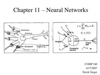
Chapter 11 – Neural Networks COMP 540 4/17/2007 Derek Singer
Motivation • Nonlinear functions of linear combinations of inputs can accurately estimate a wide variety of functions
Projection Pursuit Regression • An additive model that uses weighted sums of inputs rather than X • g,w are estimated using a flexible smoothing method • gm is a ridge function in Rp • Vm = (wm)TX is projection of X onto unit vector wm • Pursuing wm that fits model well
Projection Pursuit Regression • If M arbitrarily large, can approximate any continuous function in Rp arbitrarily well (universal approximator) • As M increases, interpretability decreases • PPR useful for prediction • M = 1: Single index model easy to interpret and slightly more general than linear regression
Fitting PPR Model • To estimate g, given w, consider M=1 model • With derived variables vi = wTxi, becomes a 1-D smoothing problem • Any scatterplot smoother (e.g. smoothing spline) can be used • Complexity constraints on g must be made to prevent overfitting
Fitting PPR Model • To estimate w, given g • Want to minimize squared error using Gauss-Newton search (second derivative of g is discarded) • Use weighted LS regression on x to find wnew • Target: Weights: • Added (w,g) pair compensates for error in current set of pairs
Fitting PPR Model • g,w estimated iteratively until convergence • M > 1, model built in forward stage-wise manner, adding a (g,w) pair at each stage • Differentiable smoothing methods preferable, local regression and smoothing splines convenient • gm’s from previous steps can be readjusted with backfitting, unclear how affects performance • wmusually not readjusted but could be • M usually estimated by forward stage-wise builder, cross-validation can also be used • Computational demands made it unpopular
From PPR to Neural Networks • PPR: Each ridge function is different • NN: Each node has the same activation/transfer function • PPR: Optimizing each ridge function separately (as in additive models) • NN: Optimizing all of the nodes at each training step
Neural Networks • Specifically feed-forward, back-propagation networks • Inputs fed forward • Errors propagated backward • Made of layers of Processing Elements (PEs, aka perceptrons) • Each PE represents the function g(wTx), g is a transfer function • g fixed, unlike PPR • Output layer of D PEs, yiÎÂD • Hidden layers, in which outputs not directly observed, are optional.
Transfer functions • NN uses parametric functions unlike PPR • Common ones include: • Threshold f(v) = 1 if v > c, else -1 • Sigmoid f(v) = 1/(1 + e-v), Range [0, 1] • Tanh f(v) = (ev – e-v)/(ev + e-v), Range [-1,1] • Desirable properties: • Monotonic, Nonlinear, Bounded • Easily calculated derivative • Largest change at intermediate values Sigmoid Hyperbolic tangent • Must scale inputs so weighted sums will fall in transition region, not saturation region (upper/lower bounds). • Must scale outputs so range falls within range of transfer function Threshold
Hidden layers • How many hidden layers and PEs in each layer? • Adding nodes and layers adds complexity to model • Beware overfitting • Beware of extra computational demands • A 3-layer network with a non-linear transfer function is capable of any function mapping.
Back Propagation Minimizing the squared error function
Learning parameters • Error function contains many local minima • If learning too much, might jump over local minima (results in spiky error curve) • Learning rates, Separate rates for each layer? • Momentum • Epoch size, # of epochs • Initial weights • Final solution depends on starting weights • Want weighted sums of inputs to fall in transition region • Small, random weights centered around zero work well
Overfitting and weight decay • If network too complex, overfitting is likely (very large weights) • Could stop training before training error minimized • Could use a validation set to determine when to stop • Weight decay more explicit, analogous to ridge regression • Penalizes large weights
Other issues • Neural network training is O(NpML) • N observations, p predictors, M hidden units, L training epochs • Epoch sizes also have a linear effect on computation time • Can take minutes or hours to train • Long list of parameters to adjust • Training is a random walk in a vast space • Unclear when to stop training, can have large impact on performance on test set • Can avoid guesswork in estimating # of hidden nodes needed with cascade correlation (analogous to PPR)
Cascade Correlation • Automatically finds optimal network structure • Start with a network with no hidden PEs • Grow it by one hidden PE at a time • PPR adds ridge functions that model the current error in the system • Cascade correlation adds PEs that model the current error in the system
Cascade Correlation • Train the initial network using any algorithm until error converges or falls under a specified bound • Take one hidden PE and connect all inputs and all currently existing PEs to it
Cascade Correlation • Train hidden PE to maximally correlate with current network error • Gradient ascent rather than descent O = # of output units, P = # of training patterns z is the new hidden PE’s current output for pattern p J = # inputs and hidden PEs connected to new hidden PE Epo is the residual error on pattern p observed at output unit o <E>, <z> are the means of E and z over all training patterns + is the sign of the term inside the abs. val. brackets
Cascade Correlation • Freeze the weights of the inputs and pre-existing hidden PEs to the new hidden PE • Weights between inputs/hidden PEs and output PEs still live • Repeat cycle of training with modified network until error converges or falls below specified bound Box = weight frozen, X = weight live
Cascade Correlation • No need to guess architecture • Each hidden PE sees distinct problem and learns solution quickly • Hidden PEs in backprop networks “engage in complex dance” (Fahlman) • Trains fewer PEs at each epoch • Can cache output of hidden PEs once weights frozen “The Cascade-Correlation Learning Architecture” Scott E. Fahlman and Christian Lebiere