Download
1 / 20
200 likes | 324 Vues
This document explores the complexities of CO2 source and sink identification using inversion modeling. It discusses forward vs. inverse modeling techniques, the current understanding of carbon fluxes, atmospheric growth rates, and the mystery of unidentified sinks. It highlights the role of human activities in carbon emissions, the uncertainties in carbon cycle feedbacks, and regional flux estimation through direct measurements at meteorological towers. The application of Bayesian inference for enhancing flux estimates is also examined, emphasizing the need for comprehensive data and robust models.

E N D
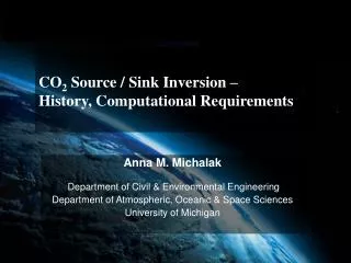
CO2 Source / Sink Inversion –History, Computational Requirements Anna M. Michalak Department of Civil & Environmental Engineering Department of Atmospheric, Oceanic & Space Sciences University of Michigan
Forward vs. Inverse Modeling Forward modeling Inverse modeling
CO2 Fluxes Present Knowledge 5.5 ± 0.3 Peta (1015 ) grams of carbon/year 3.3 ±0.2 To Atmosphere 1.6 ±0.8 Ocean Uptake Unidentified Sink Fossil Fuels Land Use Change Atmospheric Carbon To Land/Ocean 2.0 ±0.6 1.8 ± 1.5 - - = + Atmospheric Storage Uptake Human Input Source: Diane Wickland (NASA)
Global Distribution of Atmospheric Carbon Dioxide Atmospheric growth rate ~ 3 ± 0.1 Gt C/year Source: NOAA-CMDL
Where is the Missing Sink (c. 1995)? Requires uptake O2/N2, inverse modeling suggeststerrestrial Source: Kevin Gurney, CSU Northern hemisphere!!
Carbon and Climate Futures? Given nearly identical human emissions, models project dramatically different futures. Carbon cycle feedbacks are among the largest sources of uncertainty for future climate.
Spatio-temporal variability of CO2 Simulated 2-hourly column CO2Source: Olsen & Randerson (2004)
Sources of Atmospheric CO2 Information North American Carbon Program
Regional Flux Estimation Example measurement site: WLEF tall tower (447m) in Wisconsin CO2 flux measurements at: 30, 122 and 396 m CO2 mixing ratio measurements at: 11, 30, 76, 122, 244 and 396 m Photo credit: B. Stephens, UND Citation crew, COBRA
Hemispherical image from the top of the 46 meter UMBS~Flux meteorological tower Local Flux Estimation Example Measurement Site – UMBS Flux Instrumentation above the UMBS canopy is used to estimate canopy-level carbon uptake The UMBS meteorological tower is 46 m tall with gas sampling ports at 8 different heights Source: Peter Curtis, Ohio State U.
What Surface Fluxes to Atmospheric Samples See? -24 hours -48 hours -72 hours -96 hours -120 hours What Surface Fluxes to Atmospheric Samples See? 24 June 2000: Particle Trajectories Latitude Height Above Ground Level (km) Longitude Longitude Source: Arlyn Andrews, NOAA-CMDL
Linear Transport • Use transport model to generate H • Observe yat n times / locations • Invert Hto finds data transport fluxes Were the problem simple:
Need for Additional Information • Current network of atmospheric sampling sites requires additional information to constrain fluxes: • Problem is ill-conditioned • Problem is under-determined (at least in some areas) • There are various sources of error: • Measurement error • Transport model error • Aggregation error • One solution is to assimilate additional information through a Bayesian approach
Bayesian Inference Applied to Inverse Modeling for Trace Gas Surface Flux Estimation Likelihood of fluxes given atmospheric distribution Posterior probability of surface flux distribution Prior information about fluxes p(y) probabilityofmeasurements y : available observations (n×1) s: surface flux distribution (m×1)
Bayesian Formalism • Use data, y, prior flux estimates, sp, and model (with Green’s function matrix H) to estimate fluxes, s • Estimate obtained by minimizing: • Solution is • Estimates, ŝ have covariance • Residuals:
Large Regions Inversion TransCom 3 Sites & Basis Regions TransCom, Gurney et al 2003
Transport Gridscale Inversions Rödenbeck et al. 2003
Deterministic vs. Stochastic Components of Flux Estimates Remember: Xβ – Constant Component Xβ – Variable Component QHTξ ŝ (flux best estimates) January 2000
Uncertainty on Best Estimates (Variable Trend) Jan 1999 Land Jan 1999 Ocean


![[f´‚nE˘RIks]](https://cdn0.slideserve.com/1072532/f-ne-riks-dt.jpg)