Download
1 / 40
400 likes | 462 Vues
Investing in single family housing. Kevin C.H. Chiang. Outline. The determinants of home price appreciation No-arbitrage between owning and renting An application. Popular investments. Investing in single family housing is popular.

E N D
Investing in single family housing Kevin C.H. Chiang
Outline • The determinants of home price appreciation • No-arbitrage between owning and renting • An application
Popular investments • Investing in single family housing is popular. • In U.S., close to 70% of households invest in single family housing; about 30% of households rent a house or apartment. • Benefits of owning a house: financial and emotional.
Is investing in a house a good deal? • Financially speaking, yes and no. • On average, the appreciation rate based on purchase price is close to than that of T-bills. • But the built-in high leverage via mortgage can make the return on equity substantial. • If one uses the same leverage on other investments, houses suck (unconditionally). • How about conditionally? • Emotionally speaking, houses rock?
Location, location, location • The rate of price appreciation is location-specific. • During the 2004-2007 period, the median sales price of existing homes in Riverside, CA went up about 30%. • During the same period, the median sales price in Pittsburgh went down about 3%.
The determinants of appreciation • Population growth (+). • Immigration accounts for about 1/3 of U.S. population growth. • Immigrants tend to live in sunbelt cities. Sunbelt cities have been enjoyed the greatest home price appreciation. • Employment (+). • Household income (+). • Interest rate (-). • Higher interest rate = higher cost of owning a house = lower house price. • Cost of renting housing (+). • But this causality runs both way.
Asset bubble • In addition, housing prices tend to appreciate madly when the money supply is too high. • As of 01/2016.
Economic base • Regional population, employment, and income is a function of the regional economy. • Riverside had a strong economy. This lead to higher population, employment, income, and home price. • Pittsburgh ran the other way. • Thus, it is important to identify and evaluate regional economic drivers (economic base) when investing in a home.
Speculative determinants • Expectation toward appreciation. • Regulation: tax, mortgage restrictions, etc. • Example: the property tax in Hong Kong, Taiwan, and China ranges from zero to very low. It contributes to extreme high property prices in these three regions.
The supply side • The previous discussions focus on the demand side of housing. • The supply side is on average less important than the demand side: • Cost of land • Land-locked: Flagstaff. • Sea-locked: Honolulu and coastal cities. • Cost of labor • Cost of materials • Development restrictions
Submarket factors • Appreciate when net benefits are created: services received have a value greater than the taxes and fees paid for them. • A new, nice public school just built in your neighborhood. • Rezoning. • Etc.
Home price too high? Too low? • We do not have a good equilibrium asset pricing model for pricing a house. • The previous demand-supply discussions are quite general; we do not have a formula. • One way to have a formula is to use a no-arbitrage relationship: the cost of using (owning) a home = the cost of renting a home.
Cost of ownership, I • The (annual) cost of owning a house has 6 components. • 1. Opportunity cost: the cost of foregone return that the homeowner could have earned by investing in something else. • A conservative measure: the price of housing times the risk-free rate = p× rf. • 2. Cost of property taxes: p× w, where w is the property tax rate.
Cost of ownership, II • 3. The (federal) tax deductibility of mortgage interest and property taxes (-): p × × (rm + w), where is the (marginal) effective income tax rate, and rm is mortgage interest rate. • 4. Maintenance (depreciation) costs as a fraction of home value: p × . • 5. Expected capital gain/appreciation (or loss) (-): p × g, where g is the appreciation rate. • 6. An additional risk premium to compensate homeowners for the higher risk of owning versus renting: p × .
Cost of ownership, III • Annual $ cost of ownership = p× rf + p× w – p × × (rm + w) + p × – p × g + p × . • Because every term is a function of p, we can write the cost as a percentage of p (we call it the user cost of housing): • User cost = rf + w – × (rm + w) + –g +.
Cost of renting • Annual $ renting costs: R =p× r. Let us call r the rent rate, i.e., the ratio of the rent to the house price.
No-arbitrage • Annual $ renting cost = annual $ cost of owning. • R (= p× r ) = p× rf + p× w – p × × (rm + w) + p × – p × g + p × . • That is, the rent rate (the inverse of the price-to-rent ratio) must equal the user cost. • (R / p =) r = rf + w – × (rm + w) + –g +. • The lower the user cost, the higher the price-to-rent ratio.
An example • r = rf + w – × (rm + w) + –g +. • Suppose rf = 4.5%; w = 1.63% (VT); = 25%; rm = 5.5%; = 2.5%; g = 3.5%; = 2%. • The user cost = 4.5% + 1.63% – 0.25 × (5.5% + 1.63%) + 2.5% – 3.5% + 2% = 5.3475%. • For every dollar of house price, the owner pay 5.3475 cents per year in cost. • An investor will be willing to pay up to 18.7 times (1 / 0.053475) the market rent to purchase a house. • If the market rent is 4% and our inputs are correct, do houses look expensive? What if 6%?
Some analyses, I • r = rf + w – × (rm + w) + –g +. • Now, let us hold all else equal and look at one variable at a time. • If interest rates drop, what would happen to house prices? • If income tax rate is raised, what would happen to the user cost? • If investors anticipate high price appreciation, what happen to the user cost?
Some analyses, II • r = rf + w – × (rm + w) + –g +. • Suppose you buy houses and rent them out. If you expect a high price appreciation, would you accept a lower rent? • Some cities, e.g., SF, Boston, NYC, LA, have been characterized by a consistent, high price-to-rent ratio for the past several decades. Why? • This makes price-to-rent (or price-to-income) a poor measure for judging whether house prices are too high.
Appreciation rate, g • In U.S., the nominal appreciation rate is about 3.5% (this varies a lot across cities and over time), which is slightly above inflation rate. • Construction costs grow less than inflation rate. • Thus, land is appreciating faster than the structure (building). • In other words, if you would like to bet on single family housing, it may be a better idea to bet on land; surely, it is more risky.
The limitations • This analysis assumes no arbitrage. But this is not so for RE transactions. • Thus, we would expect deviations from the equality, r = rf + w – × (rm + w) + –g +. • These deviations may last for a long time (why?), but should not last forever though.
The impact of housing market on rental market • In 2007, “apartment building have been one of the few bright spots in the real estate industry as people forced out of the home-buying market by foreclosures or the credit crunch have turned to renting.” • “But now the specter of job losses is beginning to spread the gloom into that sector as well. As would-be renters are doubling up in apartments or moving in with friends and families, rent growth and occupancy rates are beginning to fall in many cities.” • Source: WSJ, Aug. 20, 2008.
An application: Beijing vs. NYC • 2015 Beijing rent rate: 2%; note that new properties in China are mostly 70-years leasehold. • 2015 NYC rent rate: 4%. • Using no-arbitrage argument, what is the most likely cause for the difference?
Recalled (from appraisal topic) • y0 = R0 + g. • Required return (yield) = cap rate + expected appreciation rate. • This is another way to understand the difference!
Meanwhile • China’s debt has quadrupled since 2007. Fueled by real estate and shadow banking, China’s total debt has nearly quadrupled, rising to $28 trillion by mid-2014, from $7 trillion in 2007. At 282 percent of GDP, China’s debt as a share of GDP, while (likely) manageable, is larger than that of the United States or Germany.
Debt to GDP ratio (x axis: change in the (%) ratio, 2007-2014)
The consequences of unrealistic expectation toward appreciation • Low cap rate? • High RE price? • Oversupply of space? Smog? • High vacancy rate? • Overly leveraged? • Default? • Bubble bursts?
Another statistic • 2015 Beijing price to income ratio: 30. • 2015 NYC price to income ratio: 10. • 2015 Los Angeles price to income ratio: 5.
More • On Sep. 4 (2013), Sunac China Holdings paid 73,000 yuan ($11,900) per buildable square meter, or about $1,100 per buildable square foot, for a residential land parcel near Beijing’s embassy district. (For comparison, the most expensive property deal in Manhattan in H1 2013 fetched $800 per buildable square foot; the average for 2012 was $323.)
03/21/2015 • (Bloomberg) -- China doesn’t need the rapid economic growth of the past and will instead focus on tasks including returning the blue to Beijing’s skies, Vice Premier Zhang Gaoli told global executives gathered in the city. • “It is both impossible and unnecessary to maintain the very high growth of the past,” said Zhang, a member of the seven-man Politburo Standing Committee, the nation’s top decision-making body. “We’ve paid the price for that,” he said Sunday. “It’s not sustainable.”
Group assignment • Please study the housing market in Burlington and neighboring cities/villages. • Please use the no-arbitrage framework to analyze the local housing market and answer the following question: is this a good time to buy a house here? • Please submit your group report in a week.
References • http://www.mckinsey.com/insights/economic_studies/debt_and_not_much_deleveraging?p=1 • http://buuea.com/looking-into-the-china-housing-market-bubble-using-gdp-and-affordability-indices/ • http://www.globalpropertyguide.com/Asia/china/Price-History • http://qz.com/121852/if-china-has-a-real-estate-glut-why-is-beijing-more-expensive-than-manhattan/ • http://www.metropolismag.com/Point-of-View/August-2013/The-Real-Problem-with-Chinas-Ghost-Towns/