Bootstrapping
This overview outlines bootstrapping methods for word sense disambiguation (WSD) and name classification using minimal supervision. The initial step involves leveraging seed examples to train a model that classifies a broader corpus. Key strategies include using confidence in classifications to iteratively refine the model, and applying the "one sense per collocation/discourse" principles to enhance accuracy. Additionally, the document discusses clustering techniques useful for natural sense identification and the efficiency of various clustering methods in the context of linguistic data analysis. ###

Bootstrapping
E N D
Presentation Transcript
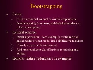
Bootstrapping • Goals: • Utilize a minimal amount of (initial) supervision • Obtain learning from many unlabeled examples (vs. selective sampling) • General scheme: • Initial supervision – seed examples for training an initial model or seed model itself (indicative features) • Classify corpus with seed model • Add most confident classifications to training and iterate. • Exploits feature redundancy in examples
Bootstrapping Decision List for Word Sense Disambiguation • Yarowsky (1995) scheme • Relies on “one sense per collocation” • Initialize seed model with all collocations in the sense dictionary definition – an initial decision list for each sense. • Alternatively – train from seed examples • Classify all examples with current model • Any example containing a feature for some sense • Compute odds ratio for each feature-sense combination; if above threshold then add the feature to the decision list • Optional: add the “one sense per discourse constraint” to add/filter examples • Iterate (2)
Results • Applies the “one sense per discourse” constraint after final classification – classify all word occurrences in a document by the majority sense • Evaluation on ~37,000 examples:
Co-training for Name Classification • Collins and Singer, EMNLP 1999 • A bootstrapping approach that relies on a (natural) partition of the feature space to two different sub-spaces • The bootstrapping process iterates by switching sub-space in each iteration • Name classification task: person, organization, location • Features for decision list: • Spelling features (full, contains, cap, non-alpha) • Context features (words, syntactic type)
Seed Features • Initialized with 0.9999 score for the decision list
DL-CoTrain Algorithm • Initialize n=5 (max. #rules learned in an iteration) • Initialize spelling decision list with seed • Classify corpus by spelling rules (where applicable) • Induce contextual rule list from classified examples; keep at most the n most frequent rules whose score>θfor each class • Classify corpus by contextual rules • Induce spelling rules, as in step 4, and add to list • If n<2500 then n n+5, and return to step 3.Otherwise, classify corpus by combined list and induce a final classifier from these labeled examples
Co-Train vs. Yarowsky’s Algorithm • Collins & Singer implemented a cautious version of Yarowsky’s algorithm, where n rules are added at each iteration • Same accuracy (~91%) (as well as a boosting-based bootstrapping algorithm) • Abney (ACL 2002) provides some analysis for both algorithm, showing that they are based on different independence assmptions
Clustering and Unsupervised Disambiguation • Word sense disambiguation without labeled training or other information sources • Cannot label to predefined senses (there are none), so try to find “natural” senses • Use clustering methods to divide different contexts of a word into “sensible” classes • Other applications of clustering: • Thesaurus construction, document clustering • Forming word classes for generalization in language modeling and disambiguation
Clustering Techniques • Hierarchical: • Bottom-up (agglomerative) • Top-down (divisive) • Flat (non-hierarchical) • Usually iterative • Soft (vs. hard) clustering • “Degree” of membership
Hierarchical: Preferable for detailed data analysis More information provided No clearly preferred algorithm Less efficient (at least O(n2)) Non-hierarchical: Preferable if efficiency is important or lots of data K-means is the simplest method and often good enough If no Euclidean space, can use EM instead Comparison
Hierarchical Clustering and but in on with for at from of to as
Similarity Functions • sim(c1,c2) = similarity between clusters • Defined over pairs of individual elements, and (possibly inductively) over cluster pairs • Values typically between 0 and 1 For hierarchical clustering, require: • Monotonicity: For all possible clusters, min[sim(c1,c2),sim(c1,c3)] sim(c1,c2 c3) Merging two clusters cannot increase similarity!
Bottom-Up Clustering Input: Set X = {x1,…,xn} of objects Similarity function sim: 2X 2X fori1 tondo: ci{xi} C {ci, ..., cn} j n + 1 while |C| > 1 do: (ca, cb) arg max(cu,cv) sim(cu,cv) cj ca cb; Trace merge to construct cluster hierarchy C (C \ {ca,cb}) {cj} j++
Types of Cluster Pair Similarity single link similarity of most similar (nearest) members complete link similarity of most dissimilar (remote) members- property of unified cluster group average average pairwise similarity of members in unified cluster- property of unified cluster
Complete Link Clustering • “Global view” yields tighter clusters – usually more suitable in NLP
Efficiency of Merge Step • Maintain pairwise similarities between clusters, and maximal similarity per cluster: • Single link update - O(n): • sim(c1 c2, c3) = max(sim(c1,c3),sim(c2,c3)) • Complete link update - O(n log(n)): • Have to compare all pairwise similarities with all points in merged cluster to find minimum
Group Average Clustering • A “mid-point” between single and complete link – produces relatively tight clusters • Efficiency depends on choice of similarity metric • Computing average similarity for a newly formed cluster from scratch is O(n2) • Goal – incremental computation • Represent objects as m-dimensional unit vectors (length-normalized), and use cosine for similarity:
Cosine Similarity cos 1 > cos 2 > cos 3 3 2 1
Efficient Cosine Similarity • Average cosine similarity within a cluster c (to be maximized after merge): • Define sum vector for cluster:
On merge, update sum: • Then update A for all new pairs of clusters • Complexity: O(n) per iteration (assuming constant dimensionality); Overall for algorithm: O(n2)
Top-Down Clustering Input: Set X = {x1,…,xn} of objects Coherence measure coh: 2X Splitting function split: 2X 2X 2X C { X } j 1 while C contains a cluster larger than 1 element do: ca arg mincucoh(cu) (cj+1,cj+2) split(ca) C (C \ ca) {cj+1,cj+2} j += 2
Top-Down Clustering (cont.) • Coherence measure – can be any type of cluster quality function, including those used for agglomerative clustering • Single link – maximal similarity in cluster • Complete link – minimal similarity in cluster • Group average – average pairwise similarity • Split – can be handled as a clustering problem on its own, aiming to form two clusters • Can use hierarchical clustering, but often more natural to use non-hierarchical clustering (see next) • May provide a more “global” view of the data (vs. the locally greedy bottom-up procedure)
Non-Hierarchical Clustering • Iterative clustering: • Start with initial (random) set of clusters • Assign each object to a cluster (or clusters) • Re-compute cluster parameters • E.g. centroids: • Stop when clustering is “good” • Q: How many clusters?
K-means Algorithm Input: Set X = {x1,…,xn} of objects Distance measure d: XX Mean function : 2XX Select k initial cluster centers f1, ..., fk while not finished do: for all clusters cjdo: cj { xi | fj = arg minf d(xi, f) } for all means fj do: fj (cj) Complexity: O(n), assuming constant number of iterations
Example Clustering of words from NY Times using cooccurring words • ballot, polls, Gov, seats • profit, finance, payments • NFL, Reds, Sox, inning, quarterback, score • researchers, science • Scott, Mary, Barbara, Edward
Buckshot Algorithm • Often, random initialization for K-means works well • If not: • Randomly choose points • Run hierarchical group average clustering:O(( )2)=O(n) • Use those cluster means as starting points for K-means • O(n) total complexity • Scatter/Gather (Cutting, Karger, Pedersen, 1993) • An interactive clustering-based browsing scheme for text collections and search results (constant time improvements)
The EM Algorithm • Soft clustering method to solve * = arg maxP(X | m()) • Soft clustering – probabilistic association between clusters and objects ( - the model parameters) Note: Any occurrence of the data consists of: • Observable variables: The objects we see • Words in each context • Word sequence in POS tagging • Hidden variables: Which cluster generated which object • Which sense generates each context • Underlying POS sequence • Soft clustering can capture ambiguity (words) and multiple topics (documents)
Two Principles Expectation: If we knew we could compute the expectation of the hidden variables (e.g, probability of x belonging to some cluster) Maximization: If we knew the hidden structure, we could compute the maximum likelihood value of
EM for Word-sense “Discrimination” Cluster the contexts (occurrences) of an ambiguous word, where each cluster constitutes a “sense”: • Initialize randomly model parameters P(vj| sk) and P(sk) • E-step: Compute P(sk | ci) for each context ci and sense sk • M-step: Re-estimate the model parameters P(vj| sk) and P(sk), for context words and senses • Continue as long as log-likelihood of all corpus contexts 1 ≤ i ≤ I increases (EM – guaranteed to increase in each step till convergence to a maximum, possibly local):
E-Step • To compute P(ci | sk), use naive Bayes assumption: • For each context i & eachsense sk, estimate the posterior probability hik = P(sk | ci) (an expected “count” of the sense for ci), using Bayes rule:
M-Step Re-estimate parameters using maximum-likelihood estimation:
Decision Procedure Assign senses by (same as Naïve Bayes): • Can adjust the pre-determined number of senses k to get finer or coarser distinctions • Bank as physical location vs. abstract corporation • If adding more senses doesn’t increase log-likelihood much, then stop
Results (Schütze 1998) Word Sense Accuracy suit lawsuit 95 0 suit you wear 96 0 motion physical movement 85 1 proposal for action 88 13 train line of railroad cars 79 19 to teach 55 33 • Works better for topic-related senses (given the broad-context features used) • Improved IR performance by 14% - representing both query and document as senses, and combining results with word-based retrieval

