The earth, ca. 1800
The earth, ca. 1800. Nevil Maskelyne and the Schiehallion experiment (1774). Schiehallion (‘Sidh Chailleann’) Scotland. Nevil Maskelyne doing his impression of Ben Franklin. d. . F. M s. m . g. F = m . g . tan( ) = G . m . M s /d 2.

The earth, ca. 1800
E N D
Presentation Transcript
Nevil Maskelyne and the Schiehallion experiment (1774) Schiehallion (‘Sidh Chailleann’) Scotland Nevil Maskelyne doing his impression of Ben Franklin d F Ms m.g F = m.g.tan() = G.m.Ms/d2 ME = (RE2/d2).(Ms/tan()) ~ 6.1024 kg RE = 6.37.106 m; VE = 1.1.1021 m3 m.g = G.m.ME/RE2 ~ 5.5 g/cm2 (initially found ~ 4.5)
Densities of common substances (all in g/cc) Ice 0.917 Water 1.000 Seawater 1.025 Graphite 2.200 Granite ~2.70 Titanium 4.507 Iron 7.870 Copper 8.960 Mercury 13.58 Gas: proportional to P/RT Two options: sub-equal mix of metal and rock or… an ideal gas, w/ high density at high P (B. Franklin)
Mass distribution in earth’s interior Period of precession Moment of inertia Period of spin Torque (sun and moon trying to pull earth’s tidal bulge into plane of ecliptic) ri I = i mi.ri2 mi Higher Earth has I much less than expected for homogeneous sphere Lower
Kraemer, 1902 View combining known density, moment of inertia, oblateness, rigidity of surface rocks, and topography Note bad for a bunch of turn-of-the-century quacks!
Earthquake nomenclature Epicenter Ground Hypocenter (‘focus’) Fault plane Other side of the earth Anticenter
Basic types of faults Ground Hanging wall Foot wall Fault plane Dip-slip (cut-away view) Normal: Hanging wall down Thrust (‘reverse’): Hanging wall up Strike-slip (bird’s eye view) Right lateral Left lateral Fault trace
0 Seconds Rupture expands circularly on fault plane, sending out seismic waves in all directions. Focus Fault cracks at surface 5 Seconds Rupture continues to expand as a crack along the fault plane. Rocks at the surface begin to rebound from their deformed state. Fault crack extends 10 Seconds The rupture front progresses down the fault plane, reducing the stress. 20 Seconds Rupture has progressed along the entire length of the fault. The earthquake stops.
The fault plane of the Landers earthquake (eastern California shear zone; 1992) Displacement on fault plane
The broader context of faulting Fault plane; episodic rupture Brittle Ca. 10-30 km deep Ductile Broad zone; continuous plastic shear
Focus “sample” outer ca. 200 km, but most energy in upper 10 km Surface waves Mantle Body waves Seismograph Core S P
Anatomy of a seismic signal Minutes 0 10 20 30 40 50 Surface waves P S ‘Primary’ (first to arrive) ‘Secondary’ (second to arrive)
P waves — analogous to sound Wave direction
S waves—analogous to light Wave direction
Surface waves Rayleigh wave (analogous to ocean surface) Wave direction Love wave (analogous to a snake or shaken rope) Wave direction
Normal modes (‘natural’ or ‘harmonic’ oscillations) Spheroidal (radial motion) Toroidal (torsional, shearing motion) On earth, periods are ca. tens of minutes
Speeds of seismic waves • Surface and normal modes have complex velocity dependencies; take 11d to learn about these! • Body waves are simpler (and more important for studying earth’s interior) elastic modulus’ (stiffness) Velocity is proportional to density (momentum) F/m2 — kg/s2m stress strain Elastic modulus = Unitless; e.g., ∂Volume/Volume Two elastic moduli: • Bulk modulus (): isotropic compression; springiness of bonds • Shear modulus (): resistance to change in shape
Speeds of seismic waves General relation: V = (modulus/)0.5 VP = ([+4/3]/)0.5 VS = (/)0.5 • For finite and , VP must be faster than VS • = 0 in fluids, so VP drops sharply and VS goes to 0 when waves hit a solid/fluid boundary
Locating the hypocenter using networks of multiple seismographs Seismograph Seismograph Epicenter Focus Seismograph
Seismogram C Seismogram B S wave Seismogram A 25 20 11-minute interval at 8600 km Time elapsed after start of earthquake (min) 8-minute interval at 5600 km 15 P wave 10 5 3-minute interval at 1500 km 0 2000 4000 6000 8000 10,000 Distance traveled from earthquake epicenter (km)
measure the amplitude of the largest seismic wave… P S Amplitude =23 mm P-wave S-wave interval = 24 seconds …and the time interval between the P- and S-waves (I.e., the distance from the epicenter. Interval between S and P waves (s) Distance (km) Connect the points to determine the Richter magnitude. Richter magnitude Amplitude (mm)
Moment magnitude Moment = Slip x Area x Elastic modulus N.meters Meters Kg/s2.m Meters2 Log10 of moment
The Mercalli Intensity scale (earthquake intensities for people who don’t like numbers and are easily scared) Board
Mg2SiO4 in upper mantle Mg2SiO4 in lower mantle
The core’s density is less than that of pure Fe. Requires a low-mass Alloying agent. S? O? H? ???