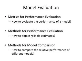
Model Evaluation
Model Evaluation. Metrics for Performance Evaluation How to evaluate the performance of a model? Methods for Performance Evaluation How to obtain reliable estimates? Methods for Model Comparison How to compare the relative performance of different models?.

Model Evaluation
E N D
Presentation Transcript
Model Evaluation • Metrics for Performance Evaluation • How to evaluate the performance of a model? • Methods for Performance Evaluation • How to obtain reliable estimates? • Methods for Model Comparison • How to compare the relative performance of different models?
Metrics for Performance Evaluation • Focus on the predictive capability of a model • Rather than how fast it takes to classify or build models, scalability, etc. • Confusion Matrix: a: TP (true positive) b: FN (false negative) c: FP (false positive) d: TN (true negative)
Metrics for Performance Evaluation… • Most widely-used metric:
Limitation of Accuracy • Consider a 2-class problem • Number of Class 0 examples = 9990 • Number of Class 1 examples = 10 • If model predicts everything to be class 0, accuracy is 9990/10000 = 99.9 % • Accuracy is misleading because model does not detect any class 1 example
Cost Matrix C(i|j): Cost of misclassifying class j example as class i
Computing Cost of Classification Accuracy = 90% Cost = 4255 Accuracy = 80% Cost = 3910
Accuracy is proportional to cost if1. C(Yes|No)=C(No|Yes) = q 2. C(Yes|Yes)=C(No|No) = p N = a + b + c + d Accuracy = (a + d)/N Cost = p (a + d) + q (b + c) = p (a + d) + q (N – a – d) = q N – (q – p)(a + d) = N [q – (q-p) Accuracy] Cost vs Accuracy
Cost-Sensitive Measures • Precision is biased towards C(Yes|Yes) & C(Yes|No) • Recall is biased towards C(Yes|Yes) & C(No|Yes) • F-measure is biased towards all except C(No|No)
Model Evaluation • Metrics for Performance Evaluation • How to evaluate the performance of a model? • Methods for Performance Evaluation • How to obtain reliable estimates? • Methods for Model Comparison • How to compare the relative performance of different models?
Methods for Performance Evaluation • How to obtain a reliable estimate of performance? • Performance of a model may depend on other factors besides the learning algorithm: • Class distribution • Cost of misclassification • Size of training and test sets
Learning Curve • Learning curve shows how accuracy changes with varying sample size • Requires a sampling schedule for creating learning curve Effect of small sample size: • Bias in the estimate • Variance of estimate
Methods of Estimation • Holdout • Reserve 2/3 for training and 1/3 for testing • Random subsampling • Repeated holdout • Cross validation • Partition data into k disjoint subsets • k-fold: train on k-1 partitions, test on the remaining one • Leave-one-out: k=n • Bootstrap • Sampling with replacement
Model Evaluation • Metrics for Performance Evaluation • How to evaluate the performance of a model? • Methods for Performance Evaluation • How to obtain reliable estimates? • Methods for Model Comparison • How to compare the relative performance of different models?
ROC (Receiver Operating Characteristic) • Developed in 1950s for signal detection theory to analyze noisy signals • Characterize the trade-off between positive hits and false alarms • ROC curve plots TPR(on the y-axis) against FPR(on the x-axis)
ROC (Receiver Operating Characteristic) • Performance of each classifier represented as a point on the ROC curve • changing the threshold of algorithm, sample distribution or cost matrix changes the location of the point
At threshold t: TP=0.5, FN=0.5, FP=0.12, FN=0.88 ROC Curve - 1-dimensional data set containing 2 classes (positive and negative) - any points located at x > t is classified as positive
ROC Curve (TP,FP): • (0,0): declare everything to be negative class • (1,1): declare everything to be positive class • (1,0): ideal • Diagonal line: • Random guessing • Below diagonal line: • prediction is opposite of the true class
Using ROC for Model Comparison • No model consistently outperform the other • M1 is better for small FPR • M2 is better for large FPR • Area Under the ROC curve • Ideal: Area = 1 • Random guess: • Area = 0.5
How to Construct an ROC curve • Use classifier that produces posterior probability for each test instance P(+|A) • Sort the instances according to P(+|A) in decreasing order • Apply threshold at each unique value of P(+|A) • Count the number of TP, FP, TN, FN at each threshold • TP rate, TPR = TP/(TP+FN) • FP rate, FPR = FP/(FP + TN)
How to construct an ROC curve Threshold >= ROC Curve:
Ensemble Methods • Construct a set of classifiers from the training data • Predict class label of previously unseen records by aggregating predictions made by multiple classifiers
Why does it work? • Suppose there are 25 base classifiers • Each classifier has error rate, = 0.35 • Assume classifiers are independent • Probability that the ensemble classifier makes a wrong prediction:
Examples of Ensemble Methods • How to generate an ensemble of classifiers? • Bagging • Boosting
Bagging • Sampling with replacement • Build classifier on each bootstrap sample • Each sample has probability 1-(1 – 1/n)nof being selected
Boosting • An iterative procedure to adaptively change distribution of training data by focusing more on previously misclassified records • Initially, all N records are assigned equal weights • Unlike bagging, weights may change at the end of boosting round
Boosting • Records that are wrongly classified will have their weights increased • Records that are classified correctly will have their weights decreased • Example 4 is hard to classify • Its weight is increased, therefore it is more likely to be chosen again in subsequent rounds
Example: AdaBoost • Base classifiers: C1, C2, …, CT • Data pairs: (xi,yi) • Error rate: • Importance of a classifier:
Example: AdaBoost • Classification: • Weight update for every iteration t and classifier j : • If any intermediate rounds produce error rate higher than 50%, the weights are reverted back to 1/n
Initial weights for each data point Data points for training Illustrating AdaBoost