
Transform and Conquer
E N D
Presentation Transcript
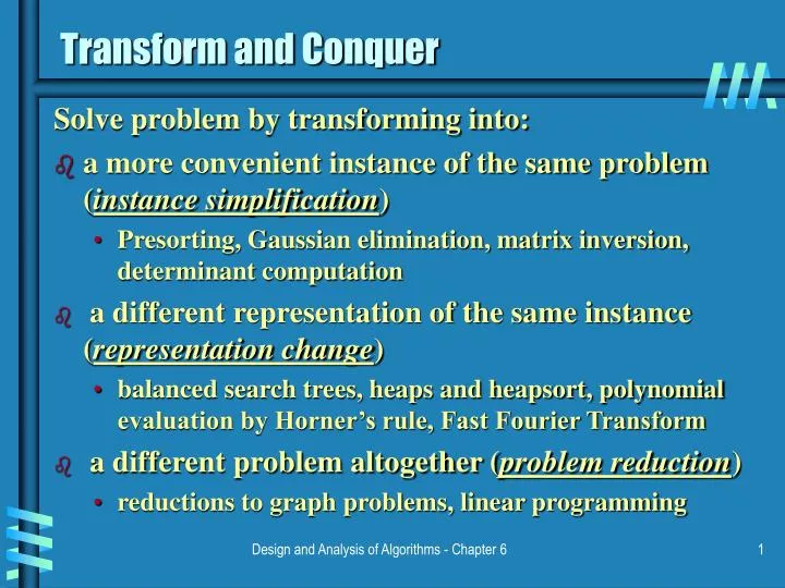
Transform and Conquer Solve problem by transforming into: • a more convenient instance of the same problem (instance simplification) • Presorting, Gaussian elimination, matrix inversion, determinant computation • a different representation of the same instance (representation change) • balanced search trees, heaps and heapsort, polynomial evaluation by Horner’s rule, Fast Fourier Transform • a different problem altogether (problem reduction) • reductions to graph problems, linear programming Design and Analysis of Algorithms - Chapter 6
Instance simplification - Presorting Solve instance of problem by transforming into another simpler/easier instance of the same problem Presorting: Many problems involving lists are easier when list is sorted. • element uniqueness • computing the mode • finding repeated elements • searching • computing the median (selection problem) Design and Analysis of Algorithms - Chapter 6
Selection Problem Find the k-thsmallest element in A[1],…A[n]. • minimum: k = 1 • maximum: k = n • median: k = n/2 • Presorting-based algorithm • sort list • return A[k] • Partition-based algorithm (decrease & conquer): • pivot/split at A[s] using partitioning algorithm • if s=k return A[s] • else if s<k repeat with sublist A[s+1],…A[n]. • else if s>k repeat with sublist A[1],…A[s-1]. Design and Analysis of Algorithms - Chapter 6
Notes on Selection Problem • Presorting-based algorithm: Ω(nlgn) + Θ(1) = Ω(nlgn) • Partition-based algorithm (decrease & conquer): • worst case: T(n) =T(n-1) + (n+1) -> Θ(n2) • best case: Θ(n) • average case: T(n) =T(n/2) + (n+1) -> Θ(n) • Bonus: also identifies the k smallest elements • Special cases max, min: better, simpler linear algorithm (brute force) • Conclusion: Presorting does not help in this case. Design and Analysis of Algorithms - Chapter 6
Finding repeated elements • Presorting-based algorithm: • use mergesort (optimal): Θ(nlgn) • scan array to find repeated adjacent elements: Θ(n) • in total it makes: Θ(nlgn) • Brute force algorithm: Θ(n2) • Conclusion: Presorting yields significant improvement Design and Analysis of Algorithms - Chapter 6
Checking element uniqueness • Brute force algorithm: Θ(n2) • Algorithm PresortedElementUniqueness Sort the array A for i 0 to n-2 do if A[i]=A[i+1] return false else return true • Conclusion: Presorting again improves • Similar improvement for mode Design and Analysis of Algorithms - Chapter 6
Checking mode • Mode is the most often met element • Brute force: scan the list and compute the frequencies. Then find the largest frequency • Algorithm PresortedMode Sort the array A i 1; modefrequency 0; while i n-1 do runlength1; runvalueA[i]; while i+runlength≤n-1 and A[i+runlength]=runvalue runlength runlength+1 if runlength> modefrequency modefrequencyrunlength, modevaluerunvalue ii+runlength return modevalue • Conclusion: Presorting again improves Design and Analysis of Algorithms - Chapter 6
Gaussian Elimination • Given a system of two linear equations with two unknowns a11x + a12y = b1 a21x + a22y = b2 • It has a unique solution unless the coefficients are proportional • Express one variable as function of the other and substitute to solve one equation. • What if the system has n equations and n unknowns ? Design and Analysis of Algorithms - Chapter 6
Gaussian Elimination (2) • Transform Ax=b to A’x=b’, where A’ upper triangular • Then, solution is possible with backward substitution • Elementary operations • Exchange equations • Replace an equation with a nonzero multiple • Replace an equation with a sum or difference of this equation and some multiple of another equation • Example 2x1 - x2 + x3 = 1 4x1 + x2 - x3 = 5 x1 + x2 + x3 = 0 Design and Analysis of Algorithms - Chapter 6
Gaussian Elimination (3) • Algorithm GaussElimination for i 1 to n do A[i,n+1]b[i] for i 1 to n-1 do for ji+1 to n do for ki to n+1 do A[j,k]A[j,k]-A[i,k]*A[j,i]/A[i,i] • Potential problems if A[i,i] is zero or very small Design and Analysis of Algorithms - Chapter 6
Gaussian Elimination (partial pivoting) • Algorithm GaussElimination2 for i 1 to n do A[i,n+1]b[i] for i 1 to n-1 do pivotrowi for ji+1 to n do if |A[j,i]|>|A[pivot,i]| pivotrowj for ki to n+1 do swap(A[i,k],A[pivotrow,k]) for ji+1 to n do tempA[j,i]/A[i,i] for kI to n+1 do A[j,k]A[j,k]-A[I,k]*temp • Efficiency Design and Analysis of Algorithms - Chapter 6
LU decomposition • Byproduct of Gaussian Elimination • Example A=LU • LUx=b. Denote y=Ux Ly=b • Solve Ly=b, then solve Ux=y • Solve with as many times with different b’s. • No extra space Design and Analysis of Algorithms - Chapter 6
Computing a matrix inverse • AA-1=I • A singular matrix does not have an inverse • A matrix is singular if and only if one of the rows is a linear combination of the other rows. • Apply Gaussian elimination. If it yields an upper-triangular with no zeros on the diagonal, then the matrix is not singular • Axj=ej Design and Analysis of Algorithms - Chapter 6
Computing the determinant • A well-known recursive formula • What if n is large ? Efficiency ? • Apply Gaussian elimination. • The determinant of an upper-triangular matrix is the product of elements on its diagonal. • Efficiency ? • Cramer’s rule Design and Analysis of Algorithms - Chapter 6
Taxonomy of Searching Algorithms • Elementary searching algorithms • sequential search • binary search • binary tree search • Balanced tree searching • AVL trees • red-black trees • multiway balanced trees (2-3 trees, 2-3-4 trees, B trees) • Hashing • separate chaining • open addressing Design and Analysis of Algorithms - Chapter 6
Balanced trees: AVL trees • For every node, difference in height between left and right subtree is at most 1 • AVL property is maintained through rotations, each time the tree becomes unbalanced • lg n≤h≤ 1.4404 lg (n + 2) - 1.3277 average: 1.01 lg n + 0.1 for large n • Disadvantage: needs extra storage for maintaining node balance • A similar idea: red-black trees (height of subtrees is allowed to differ by up to a factor of 2) Design and Analysis of Algorithms - Chapter 6
AVL tree rotations • Small examples: • 1, 2, 3 • 3, 2, 1 • 1, 3, 2 • 3, 1, 2 • Larger example: 4, 5, 7, 2, 1, 3, 6 • See figures 6.4, 6.5 for general cases of rotations; Design and Analysis of Algorithms - Chapter 6
General case: single R-rotation Design and Analysis of Algorithms - Chapter 6
Double LR-rotation Design and Analysis of Algorithms - Chapter 6
Balance factor • Algorithm maintains balance factor for each node. For example: Design and Analysis of Algorithms - Chapter 6
Heapsort Definition: A heap is a binary tree with the following conditions: • it is essentially complete: • The key at each node is ≥ keys at its children Design and Analysis of Algorithms - Chapter 6
Definition implies: • Given n, there exists a unique binary tree with n nodes that is essentially complete, with h= lg n • The root has the largest key • The subtree rooted at any node of a heap is also a heap Design and Analysis of Algorithms - Chapter 6
Heapsort Algorithm: • Build heap • Remove root –exchange with last (rightmost) leaf • Fix up heap (excluding last leaf) Repeat 2, 3 until heap contains just one node. Design and Analysis of Algorithms - Chapter 6
Heap construction • Insert elements in the order given breadth-first in a binary tree • Starting with the last (rightmost) parental node, fix the heap rooted at it, if it does not satisfy the heap condition: • exchange it with its largest child • fix the subtree rooted at it (now in the child’s position) Example: 2 3 6 7 5 9 Design and Analysis of Algorithms - Chapter 6
Root deletion The root of a heap can be deleted and the heap fixed up as follows: • exchange the root with the last leaf • compare the new root (formerly the leaf) with each of its children and, if one of them is larger than the root, exchange it with the larger of the two. • continue the comparison/exchange with the children of the new root until it reaches a level of the tree where it is larger than both its children Design and Analysis of Algorithms - Chapter 6
1 2 3 4 5 6 9 5 3 1 4 2 Representation • Use an array to store breadth-first traversal of heap tree: • Example: • Left child of node j is at 2j • Right child of node j is at 2j+1 • Parent of node j is at j /2 • Parental nodes are represented in the first n /2 locations 9 5 3 1 4 2 Design and Analysis of Algorithms - Chapter 6
Bottom-up heap construction algorithm Design and Analysis of Algorithms - Chapter 6
Analysis of Heapsort See algorithm HeapBottomUp in section 6.4 • Fix heap with “problem” at height j: 2j comparisons • For subtree rooted at level i it does 2(h-i) comparisons • Total for heap construction phase: h-1 Σ 2(h-i) 2i = 2 ( n – lg (n + 1)) = Θ(n) i=0 # nodes at level i Design and Analysis of Algorithms - Chapter 6
Analysis of Heapsort (continued) Recall algorithm: • Build heap • Remove root –exchange with last (rightmost) leaf • Fix up heap (excluding last leaf) Repeat 2, 3 until heap contains just one node. Θ(n) Θ(log n) n – 1 times Total:Θ(n) + Θ( n log n) = Θ(n log n) • Note: this is the worst case. Average case also Θ(n log n). Design and Analysis of Algorithms - Chapter 6
Priority queues • A priority queue is the ADT of an ordered set with the operations: • find element with highest priority • delete element with highest priority • insert element with assigned priority • Heaps are very good for implementing priority queues Design and Analysis of Algorithms - Chapter 6
Insertion of a new element • Insert element at last position in heap. • Compare with its parent and if it violates heap condition exchange them • Continue comparing the new element with nodes up the tree until the heap condition is satisfied Example: Efficiency: Design and Analysis of Algorithms - Chapter 6
Bottom-up vs. Top-down heap construction • Top down: Heaps can be constructed by successively inserting elements into an (initially) empty heap • Bottom-up: Put everything in and then fix it • Which one is better? Design and Analysis of Algorithms - Chapter 6
Horner’s rule • Horner published in early 19th century • According to Knuth, the method was used by Newton • Evaluate a polynomial at a point x p(x) = anxn + an-1xn-1 + … + a1x + a0 p(x) = ( … (anx + an-1) x + … )x + a0 • Example: evaluate p(x)=2x4-x3+3x2+x-5 at x=3 p(x) = x (x (x (2x-1) + 3) + 1) - 5 • Visualization by a table Design and Analysis of Algorithms - Chapter 6
Horner’s rule [2] • Algorithm Horner(P[0..n],x) // Evaluate polynomial at a given point // Input: an array P[0..n] of coefficients and a number x //Output: the value of polynomial at point x p P[n] for i n-1 down to 0 do p x*p + P[i] return p • Efficiency ? • Byproduct: coefficients of the quotient of the division of p(x) by (x-x0) Design and Analysis of Algorithms - Chapter 6
Binary exponentiation • Horner is not efficient to compute p(x)=xn at x=a • Degenerate to brute force • Let the binary representation n=blbl-1… bi … b1b0 • p(x) = blxl + bl-1xl-1 + … + b1x + b0 and x=2 • Algorithm LeftRightBinaryExponentiation product a for i l-1 down to 0 do product product * product if bi1 then product product*a return product • Example: compute a13, n=13=1101 • Efficiency Design and Analysis of Algorithms - Chapter 6
Binary exponentiation (2) • Compute an • Consider n = bl2l + bl-12l-1 + … + b12 + b0 and multiply independent powers terms • Algorithm RightLeftBinaryExponentiation term a if b0=1 then product a else product 1 for i 1 to l do term term * term if bi = 1 then product product * term return product • Example: compute a13, n=13=1101 • Efficiency Design and Analysis of Algorithms - Chapter 6
Least common multiple • lcm(24,60)=120, lcm(11,5)=55 • Example: 24 = 2 x 2 x 2 x 3 60 = 2 x 2 x 3 x 5 lcm(24,60) = (2x2x3) x 2 x 5 • Efficiency (a list of primes is required) • lcm(m,n) = mn / gcd(m,n) Design and Analysis of Algorithms - Chapter 6
Counting paths in a graph • The number of different paths of length k>0 from node i to node j equals the (i,j) element of the Ak, where A the adjacency matrix • Example • Efficiency Design and Analysis of Algorithms - Chapter 6
Reduction to graph problems • Applies for a variety of games and puzzles • Build the state-space graph • Example: peasant, wolf, goat, cabbage • Traverse the graph by applying what? Design and Analysis of Algorithms - Chapter 6