SIMPLE AND MULTIPLE REGRESSION
1.07k likes | 1.13k Vues
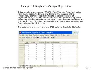
Analyzing the relationship between variables in the PISA 2003 dataset using regression analysis. Explore correlations, regressions, and data visualization techniques to understand connections between math performance and various factors. Detailed syntax and examples are provided for SPSS and R software.

SIMPLE AND MULTIPLE REGRESSION
E N D
Presentation Transcript
Relació entre variables Entre variables discretes (exemple: veure Titanic) Entre continues (Regressió !) Entre discretes i continues (Regressió!)
Pisa 2003 > Rendiment en Matemàtiques, > Nombre de llibres a casa
Pisa 2003 > Rendiment en Matemàtiques, > Nombre de llibres a casa
Regressió Lineal ? Pisa 2003
Regressió Lineal ? Pisa 2003
Regressió Lineal ? Pisa 2003
* We first load the PISAespanya.sav file and then * this is the sintaxis file for SPSS analysis *Q38 How often do these things happen in your math class *Student dont't listen to what the teacher says CROSSTABS /TABLES=subnatio BY st38q02 /FORMAT= AVALUE TABLES /STATISTIC=CHISQ /CELLS= COUNT ROW . FACTOR /VARIABLES pv1math pv2math pv3math pv4math pv5math pv1math1 pv2math1 pv3math1 pv4math1 pv5math1 pv1math2 pv2math2 pv3math2 pv4math2 pv5math2 pv1math3 pv2math3 pv3math3 pv4math3 pv5math3 pv1math4 pv2math4 pv3math4 pv4math4 pv5math4 /MISSING LISTWISE /ANALYSIS pv1math pv2math pv3math pv4math pv5math pv1math1 pv2math1 pv3math1 pv4math1 pv5math1 pv1math2 pv2math2 pv3math2 pv4math2 pv5math2 pv1math3 pv2math3 pv3math3 pv4math3 pv5math3 pv1math4 pv2math4 pv3math4 pv4math4 pv5math4 /PRINT INITIAL EXTRACTION FSCORE /PLOT EIGEN ROTATION /CRITERIA FACTORS(1) ITERATE(25) /EXTRACTION ML /ROTATION NOROTATE /SAVE REG(ALL) . GRAPH /SCATTERPLOT(BIVAR)=st19q01 WITH fac1_1 /MISSING=LISTWISE . REGRESSION /MISSING LISTWISE /STATISTICS COEFF OUTS R ANOVA /CRITERIA=PIN(.05) POUT(.10) /NOORIGIN /DEPENDENT fac1_1 /METHOD=ENTER st19q01 /PARTIALPLOT ALL /SCATTERPLOT=(*ZRESID ,*ZPRED ) /RESIDUALS HIST(ZRESID) NORM(ZRESID) .
library(foreign) help(read.spss) data=read.spss("G:/DATA/PISAdata2003/ReducedDataSpain.sav", use.value.labels=TRUE,to.data.fram=TRUE) names(data) [1] "SUBNATIO" "SCHOOLID" "ST03Q01" "ST19Q01" "ST26Q04" "ST26Q05" [7] "ST27Q01" "ST27Q02" "ST27Q03" "ST30Q02" "EC07Q01" "EC07Q02" [13] "EC07Q03" "EC08Q01" "IC01Q01" "IC01Q02" "IC01Q03" "IC02Q01" [19] "IC03Q01" "MISCED" "FISCED" "HISCED" "PARED" "PCMATH" [25] "RMHMWK" "CULTPOSS" "HEDRES" "HOMEPOS" "ATSCHL" "STUREL" [31] "BELONG" "INTMAT" "INSTMOT" "MATHEFF" "ANXMAT" "MEMOR" [37] "COMPLRN" "COOPLRN" "TEACHSUP" "ESCS" "W.FSTUWT" "OECD" [43] "UH" "FAC1.1" attach(data) mean(FAC1.1) [1] -8.95814e-16 tabulate(ST19Q01) [1] 106 0 15 1266 1927 2372 3575 1155 375 > table(ST19Q01) ST19Q01 Miss Invalid N/A More than 500 books 106 0 15 1266 201-500 books 101-200 books 26-100 books 11-25 books 1927 2372 3575 1155 0-10 books 375
Data Variables Y and X observed on a sample of size n: yi , xi i =1,2, ..., n
Coeficient de correlació r = 0 , tot i que hi ha una relació funcional exacta (no lineal!) > cbind(x,y) x y [1,] -10 100 [2,] -9 81 [3,] -8 64 [4,] -7 49 [5,] -6 36 [6,] -5 25 [7,] -4 16 [8,] -3 9 [9,] -2 4 [10,] -1 1 [11,] 0 0 [12,] 1 1 [13,] 2 4 [14,] 3 9 [15,] 4 16 [16,] 5 25 [17,] 6 36 [18,] 7 49 [19,] 8 64 [20,] 9 81 [21,] 10 100 >
Regressió Lineal Simple Variables Y X E Y | X = a + b X Var (Y | X ) = s2
Regression Model Yi = a + b Xi + ei ei : mean zero variance s2 normally distributed
Fitted regression line a= 0.5789 b=0.6270
Fitted and true regression lines: a=1, b=.6 a= 0.5789 b=0.6270
Fitted and true regression lines in repeated (20) sampling a=1, b=.6
OLS estimate of beta (under repeated sampling) Estimate of beta for different samples (100): 0.619 0.575 0.636 0.543 0.555 0.594 0.611 0.584 0.576 ...... > a=1, b=.6 > mean(bs) [1] 0.6042086 > sd(bs) [1] 0.03599894 >
REGRESSION Analysis of the Simulated Data (with R and other software )
Fitted regression line: a=1, b=.6 a= 1.0232203, b= 0.6436286
Regression Analysis regression = lm(Y ~X) summary(regression) Call: lm(formula = Y ~ X) Residuals: Min 1Q Median 3Q Max -6.0860 -2.1429 -0.1863 1.9695 9.4817 Coefficients: Estimate Std. Error t value Pr(>|t|) (Intercept) 1.0232 0.3188 3.21 0.00180 ** X 0.6436 0.0377 17.07 < 2e-16 *** --- Signif. codes: 0 `***' 0.001 `**' 0.01 `*' 0.05 `.' 0.1 ` ' 1 Residual standard error: 3.182 on 98 degrees of freedom Multiple R-Squared: 0.7483, Adjusted R-squared: 0.7458 F-statistic: 291.4 on 1 and 98 DF, p-value: < 2.2e-16 >>
Regression Analysis with Stata . use "E:\Albert\COURSES\cursDAS\AS2003\data\MONT.dta", clear . regress y x Source | SS df MS Number of obs = 100 ---------+------------------------------ F( 1, 98) = 291.42 Model | 2950.73479 1 2950.73479 Prob > F = 0.0000 Residual | 992.280727 98 10.1253135 R-squared = 0.7483 ---------+------------------------------ Adj R-squared = 0.7458 Total | 3943.01551 99 39.8284395 Root MSE = 3.182 ------------------------------------------------------------------------------ y | Coef. Std. Err. t P>|t| [95% Conf. Interval] ---------+-------------------------------------------------------------------- x | .6436286 .0377029 17.071 0.000 .5688085 .7184488 _cons | 1.02322 .3187931 3.210 0.002 .3905858 1.655855 ------------------------------------------------------------------------------ . predict yh . graph yh y x, c(s.) s(io)
Fitted Regression FYi = 1.02 + .64 Xi , R2=.74 s.e.: (.037) t-value: 17.07 Regression coeficient of X is significant (5% significance level), with the expected value of Y icreasing .64 for each unit increase of X. The 95% confidence interval for the regression coefficient is [.64-1.96*.037, . .64+1.96*.037]=[.57, .71] 74% of the variation of Y is explained by the variation of X
Interpreting multiple regression by means of simple regression
Exemple de l’Anàlisi de Regressió Dades de paisos.sav