Download
1 / 1
10 likes | 120 Vues
This study utilizes the resources of the White Rose Grid and UK MHD consortium to conduct numerical simulations of acoustic wave propagation in the solar sub-photosphere, influenced by a localized magnetic field concentration. We successfully balanced computations between ICEBERG at Sheffield and the MHD CLUSTER at St. Andrews, allowing for efficient processing of data. Initial equilibrium conditions were derived from standard solar models and prepared at ICEBERG, followed by detailed acoustic response analyses at St. Andrews using an MPI parallel MHD code. The results unveil the complex interaction of sound waves with magnetic fields in a gravitationally stratified plasma.

E N D
Numerical simulations of sound waves in the magnetised solar sub-photosphere using the resources of WRG and UK MHD consortium S. Shelyag, S. Zharkov, V. Fedun, R. Erdélyi, M.J. Thompson Solar Physics and Space Plasma Research Centre (SP2RC), Department of Applied Mathematics, University of Sheffield, Sheffield, UK Using the resources of White Rose Grid and UK MHD consortium, we have been able to perform numerical simulations of acoustic wave propagation and dispersion in the solar subphotosphere with a localized magnetic field concentration. By distributing computations between ICEBERG (Sheffield) and MHD CLUSTER in St Andrews, we achieved reasonable performance and computational time. We used ICEBERG to prepare the initial equilibrium density and pressure stratifications, which are derived from a standard solar model, and to adjust magnetohydrostatic and convective stability. The initial data is transferred to St Andrews, where our MPI parallel MHD code takes it as the initial condition and produces raw acoustic response data. Then the data is transferred back to ICEBERG, where time-distance diagrams of the vertical velocity perturbation at the level corresponding to the visible solar surface are produced and visualization is performed. 1. Usage of the resources Local Computer ICEBERG St Andrews MHD cluster INITIAL MODEL INITIAL DATA DATA PREPARATION ROUTINE PARALLEL MHD CODE VISUALIZATION DATA RAW OUTPUT DATA VISUALIZATION SOFTWARE Fig.1. The data flow in the designed simulation system. Initial one-dimensional standard solar model is prepared using the Local Computer. Then, using the Data Preparation Routine at ICEBERG, the model is transformed to the two-dimensional plane parallel initial data snapshot, which is then used at St Andrews MHD cluster as an initial condition for the MPI Parallel MHD Code. Raw data containing the calculation results is transported back to ICEBERG where the visualization software is used to reduce and analyze the data. 2. MPI parallel MHD code 3. Sunspot configuration We use a self-similar non-potential magnetic field configuration, which can be obtained from the following set of equations (Schlüter and Temesváry, 1958; Schüssler and Rempel, 2005; Cameron et al., 2008). This magnetic field is divergence free by definition. Pressure and density are then recalculated numerically using the magnetohydrostatic equilibrium condition. We have developed the Sheffield Advection Code SAC that allows us to simulate the interaction of any arbitrary perturbation (not necessarily limited to the linearised regime) with the background plasma in magnetohydrostatic equilibrium. Hyperdiffusion and hyperresistivity are implemented to achieve numerical stability of the computed solution of the MHD equations. We found more complex form of the MHD equations especially suitable for numerical simulations of processes in a stable gravitationally-stratified plasma and implemented them on the base of the well-known Versatile Advection Code. Our code exploits Message Passing Interface standard, uses a domain decomposition scheme for parallelization purposes and is suitable for use at St Andrews MHD cluster. Full description of the code, details of the implemented methods and tests can be found in Shelyag et al. (2008). Fig.2. Magnetic field configuration. The vertical and horizontal components of the magnetic field are shown to the left. The field lines are overplotted. This configuration mimics a sunspot, where the magnetic field is essentially non-uniform. 4. Model responce 5. Time-distance diagram We introduce a perturbation source described by the expression: Fig.4. Vertical component of velocity taken at the 250 km depth as a function of time. The first, second and third bounces are clearly visible on the time-distance diagram.A weak reflection of the wave from the side boundaries can also be noticed. No noticeable influence of the magnetic field can be seen. This will be revealed in the next section. 1 2 3 where T0=300 s, T1=600 s, σ1=100 s, σ2=0.1 Mm, r0 is the source location. Fig.3. Power spectrum of the vertical velocity perturbation generated by the source. The p modes are visible up to high orders. Eigenmodes of the background model are overplotted by solid lines. 6. Time-distance difference 6. Results Fig. 5. Vertical speed difference images. The differences are computed between the points located at the same distance and opposite sides from the source. The first bounce is affected only locally by the magnetic field, however, the second and third bounces are also affected in the 60-80 Mm distance region. We have discussed the use of UK White Rose Grid and the resources of UK MHD consortium for solar MHD and helioseismological simulations. We simulated and analyzed the influence of the magnetic field on the acoustic response of the simulated solar sub-photosphere. Fig. 5 shows the difference in sound wave propagation between the horizontally homogeneous non-magnetic and the non-uniform magnetic regions of the simulation domain. The temperature increase below the simulated sunspot causes negative phase shifts of the wave packets propagating through it. 1 2 3 References: Cameron R., et al, 2008, Solar Physics, in press Schlüter A., Temesváry, S., IAUS 6, 263, 1958 Schüssler M., Rempel, M., A&A, 2005, 441, 337 Shelyag, S., et al. A&A, 486, 655, 2008