Download
1 / 54
540 likes | 640 Vues
Explore hysteresis, bistable behavior, and the tipping point in natural systems. Understand how systems oscillate between states and the mechanisms governing state changes.

E N D
The Kind of Problem the Environment Is 4. Bistable Behavior Lynn S. Fichter • Department of Geology/Environmental Science • E-mail: fichtels@jmu.edu • James Madison University • http://csmres.jmu.edu/geollab/Fichter/Fichter/Fichterls.html • Fall, 2007 • http://www.jmu.edu/geology/evolutionarysystems/Academy2005.shtml
The Ubiquity of Oscillating Systems in the World One of the very common phenomena in the world are systems that oscillates between two or more states, like . . . 1 The, the daily heating and cooling cycle, 2 Or, the seasonal cycles, 3 Or cycles of populations, 4 Or waves of economic expansion followed by recession. 5 Or, sleeping and waking.
Oscillating Systems Or, as in the logistic system
Oscillating Systems Or, as in the Lorenz strange attractor system Run Lorenz Attractor Lorenz Applet http://www.csounds.com/mastering/em_10.html http://www.cmp.caltech.edu/~mcc/chaos_new/Lorenz.html
Oscillating Systems Which leads to the more pertinent question - when a system has more than one path available to it, and periodically switches between them, when and how does it choose to make the switch? Here we see the ability of a system to exist in different states under the same conditions (i.e. same r value).
Hysteresis a.k.a. Bistable Behavior Has two different meanings, and we need to understand both. 1. The lag in response between a cause and its effect. AND 2. The ability of a system to exist in different states under the same conditions.
Hysteresis as the Lag Between Cause and Effect The sand pile builds . . . grain . . . by grain . . . by grain . . . by grain . . . by grain . . . by grain . . . by grain . . . by grain . . . Description One Building toward the critical state . . . Where it avalanches building building building avalanche avalanche avalanche Thus we see there is a lag between cause (accumulation of individual sand grains), and the effect (avalanche).
Hysteresis as the Lag Between Cause and Effect Fractal sand supply Now, imagine the sand supply follows a power law (or is fractal), with different numbers of grains falling at different times. Avalanches will also be fractal, and follow a power law distribution. Earth Temp. curve over the past 400,000 years http://atlas.gc.ca/maptexts/topic_texts/english/images/TemperatureCO2.jpg
State 1 Bistable Variable State 2 Driving Variable Bistable – How a System Can Exist In Distinctly Different States Under the Same Conditions Over shoots left Over shoots right Over shoots left Over shoots right Description Two X = dependent variable Time Series Hysteresis Diagram r = independent variable
Bistable – How a System Can Exist In Distinctly Different States Under the Same Conditions First, a little slight of hand . . . State 1 Time Series is now the Bistable Variable Time Series at one “r” value “r” is still the external energy driving the system State 2 X as Dependent Variable X is now the Driving Variable Bistable behavior requires that two variables be coupled in a positive/negative feedback loop. • A rise in one variable causes the other variable to fall, and vice versa. • Cannot speak of independent and dependent variables since they are coupled.
Mechanisms of Bistable Behavior High Bistable Variable Low Driving Variable How the system “decides” to change from one state to another System begins here; high Bistable, low Driving Driving Variable is driven to the right (by the external energy of “r”) Description Three On this path Driving variable has mostly small effects on Bistable. But system is building to critical state. Tipping Point: system has built to the critical state System now driven left
Mechanisms of Bistable Behavior How the system “decides” to change from one state to another The Tipping Point The prevalence of this phenomena of lags between cause and effect was explored by Malcolm Gladwell in “The Tipping Point” "The best way to understand the dramatic transformation of unknown books into bestsellers, or the rise of teenage smoking, or the phenomena of word of mouth or any number of the other mysterious changes that mark everyday life, is to think of them as epidemics. Ideas and products and messages and behaviors spread just like viruses do." Little changes can have big effects; when small numbers of people start behaving differently, that behavior can ripple outward until a critical mass or "tipping point" is reached, changing the world. Return to Systems
Mechanisms of Bistable Behavior High Bistable Variable Low Driving Variable How the system “decides” to change from one state to another System begins here; high Bistable, low Driving Driving Variable is driven to the right (by an external variable) Here Driving has small effects on Bistable. But system is building to critical state. But, system cannot go down this path because there are no stable states here Tipping Point: small change in Driving has large effect on Bistable (i.e. is sensitive dependent). System now driven left
Mechanisms of Bistable Behavior How the system “decides” to change from one state to another System now driven left
Mechanisms of Bistable Behavior High Bistable Variable Low Driving Variable How the system “decides” to change from one state to another System begins here; high Bistable, low Driving Driving Variable is driven to the right (by an external variable) Here Driving has small effects on Bistable. But system is building to critical state. Tipping Point: small change in Driving has large effect on Bistable. In here there are no stable states Tipping Point: So system avalanches to a low state on the Bistable variable System cannot return to upper path from here but must be driven left first (because high Driving variable is not stable under low Bistable variable). System now driven left
Stability of the Bistable System The bistable behavior is stable only within a narrow range of “r” values. If one variable comes to dominate the system, the system either goes runaway negative feedback (closes down to point attractor, or an earlier state), or run away positive feedback (chaos). Increase external driving force and system bifurcates to different attractor Lower external driving force, and system closes down System now driven left
Hysteresis Caveats: warnings and cautions Hysteresis loop describes the behavior of the system . . . State 1 It does not explain the cause-effect relationships behind the behavior. Bistable Variab le And it does not explain the source of the energy driving everything. State 2 These systems are driven by processes and energy sources outside the diagram. Driving Variable • Ultimately things like social stresses, fear, bigotry, economic gyrations, etc. • The hysteresis Driving Variable is itself being driven. • Or, “everything is connected with everything else by positive and negative feedback.” • We can isolate the bistable system to discern the relationships among the variables, but what keeps the system “open” with enough “r” value comes from outside the system.
Bistable Behavior Social/Economic Example Paul Ormerod
Bistable Behavior Social/Economic Example How the proportion of criminals in a population varies with the level of social and economic deprivation Begin here: high deprivation, high crime For any given reduction in deprivation the impact on crime becomes stronger. But, not until the tipping point does the frequency of crime drop dramatically. Percentage of population who become criminals Tipping Point: Level of social and economic deprivation At the tipping point even a very small further reduction in the level of deprivation leads to dramatically lower crime rates. Once we are on the bottom line, additional falls in deprivation reduce crime by only small amounts.
Bistable Behavior Social/Economic Example How the proportion of criminals in a population varies with the level of social and economic deprivation Begin here: high deprivation, high crime For any given reduction in deprivation the impact on crime becomes stronger. But, not until the tipping point does the frequency of crime drop dramatically. Percentage of population who become criminals Tipping Point: Level of social and economic deprivation At the tipping point even a very small further reduction in the level of deprivation leads to dramatically lower crime rates. Once we are on the bottom line, additional falls in deprivation reduce crime by only small amounts.
Example of Bistable Behavior How the proportion of criminals in a population varies with the level of social and economic deprivation The bistable nature is illustrated by today when the country is rather prosperous, but crime levels are very high, in contrast with the depression of the 1930’s, when deprivation was very high, but crime was low. Liberal Explanation At the tipping point the level of deprivation is high enough that lots of people turn to crime just to survive Percentage of population who are criminals Tipping Point: Level of Social and Economic Deprivation Once on the bottom line crime remains low, or rises only very slowly even as the level of economic deprivation continues to rise.
Example of Bistable Behavior How the severity of the criminal justice system affects the level of crime in the population. We assume that the effect of a more punitive criminal justice system is to reduce the proportion of criminals in the population. As the criminal justice system becomes more strict the proportion of criminals in the population falls. But the effect at first is rather minimal. Conservative Explanation Now the cost of crime is so low many people return to crime (out of greed?). At Tipping Point punishment is high enough it dissuades non-hard-core criminals from committing crimes. Percentage of population who are criminals Crime rates fall dramatically. As punishment laxes crime slowly increases (because crime has low cost) Severity of Criminal Justice
Neither the conservative nor the liberal explanations are complete and adequate explanations. Social economic deprivation One group controls another positive feedback loop positive feedback loop Job Availability Prevalent feelings of loss of personal control and responsibility. Cultural & political crisis Need to place blame for misfortune elsewhere “The world is one. It is a unity. Nothing is separate, everything pulsates together. We are joined with each other, interlinked.”
Neither the conservative nor the liberal explanations are complete and adequate explanations. Social economic deprivation One group controls another positive feedback loop positive feedback loop Job Availability Prevalent feelings of loss of personal control and responsibility. Cultural & political crisis Need to place blame for misfortune elsewhere The world is also a complex system and does not behave in the ways classical science studies.
Bistable Behavior A Geological Example Glacial/Interglacial Cycles
Bistable Behavior Snowball Earth - A Geological Example Between 750 – 580 million years ago Earth underwent four extremely severe, global-wide, glaciation events, each lasting about 10 million years. No ice, lots of land, low albedo (sunlight absorbed, not reflected). Earth warm. Reflective cooling (albedo) leads to more ice, which increases albedo even more, which leads to runaway positive feedback. Earth cools even more quickly. CO2 removed from atmosphere by weathering of vast open land areas, reducing greenhouse effect. Negative feedback on warm conditions; Earth cools. Snowball Earth: cooling maximized (-50o C below zero). Entire Earth, including oceans, frozen solid. CO2 cooling leads to ice formation, which increases albedo which increases cooling; + feedback = increased cooling.
Bistable Behavior in Bifurcation Diagrams A Geological Example Glacial/Interglacial Cycles Cooling Part of Cycle High Weathering removes CO2 which leads to ice, which increases albedo When continents are exposed, abundant weathering of exposed rock sucks down CO2 from atmosphere, slowly at first but with increasing effect with time. Earth Temperature • Lower CO2 concentrations in atmosphere lowers the greenhouse effect of CO2 leading to cooling. Earth descends into and gets locks in Snowball Earth Low High Atmospheric CO2 Low • When it is cool enough for ice sheets to begin forming the increasing albedo causes temp-erature to drop even more. Albedo (ice reflection of sunlight) becomes a positive feedback system driving Earth deeper and deeper into the ice age.
This is the way the world ends This is the way the world ends This is the way the world ends Not with a bang but a whimper. The Hollow Men T. S. Eliot (1925)
Bistable Behavior A Geological Example Reversal of Snowball Earth There is no extrinsic reason for Snowball Earth to have come to an end. Once locked into the positive feedback loop of cooling, leading to more cooling, leading to more cooling the Earth should have become stuck there. The reason it did not become stuck was Intrinsic, the Earth is an open, dissipative system, and what it dissipates is tectonic energy – energy from its molten interior.
Bistable Behavior A Geological Example Reversal of Snowball Earth The interior of the Earth was still molten hot. Volcanoes still spewed CO2 gas through the glacial ice into the atmosphere. Which reduced the albedo, which led to more warming, which led to more ice melting, which lead to lower albedo, etc., etc., etc. Because there was no exposed land there was no weathering to suck down the CO2 , so . . . Accumulating atmospheric CO2 increased greenhouse atmospheric warming until it was warm enough for the ice to begin to melt. http://earthobservatory.nasa.gov/Newsroom/NewImages/images_topic.php3?img_id=16833&topic=heat
Bistable Behavior A Geological Example Reversal of Snowball Earth Warming Part of Cycle High Weathering removes CO2 Expanded ice sheets lead to rise of CO2 in atmosphere. This cycle took about 10 million years Rapid warming • Ice sheets decrease area of exposed rock, reducing weathering rates, decreasing loss of CO2 from atmosphere. Earth Temperature • Ongoing volcanic outgassing puts CO2 back into atmosphere. Rising CO2 builds to tipping point Low High Atmospheric CO2 Low At first these trends have minimal effect on Earth Temperature. But, when CO2 rises high enough its concentration in the atmosphere crosses a threshold leading to rapid warming trends leading to glacial melting. Return to Systems
Bistable Behavior in Recent Climate A Geological Example Pleistocene Glacial/Interglacial Cycles Bard E. Abrupt climate changes over millennial time scales: climate shock. Physics Today 55, 32-37 (2002) (link) Return to Systems http://www.cerege.fr/tracorga/BARD/bard89.html
NOA Oscillation ENSO La Nina and El Nino Oscillation
Deep Freeze Conditions Warm Conditions Bistable Behavior in Recent Climate The North Atlantic Oscillation Recent Glacial/Interglacial Cycles El Nino Southern Oscillation http://www.isse.ucar.edu/signal/15/articles.html http://sinus.unibe.ch/klimet/wanner/nao.html
The Southern Oscillation El Nino and La Nina Near the end of each year as the southern hemispherical summer is about to peak, a weak, warm counter-current flows southward along the coasts of Ecuador and Peru, replacing the cold Peruvian current. Centuries ago the local residents named this annual event El Niño (span. "the child") based on Christian theology that assigned this period of the year the name-giving Christmas season. Normally, these warm countercurrents last for at most a few weeks when they again give way to the cold Peruvian flow. However, every three to seven years, this countercurrent is unusually warm and strong. Accompanying this event is a pool of warm, ocean surface water in the central and eastern Pacific. El Niño has made frequent appearances over the last century, with particularly severe consequences in 1891, 1925, 1953, 1972, 1982, 1986, 1992, 1993, and 1997. http://www.sbg.ac.at/ipk/avstudio/pierofun/atmo/elnino.htm
The Southern Oscillation El Nino and La Nina http://www.sbg.ac.at/ipk/avstudio/pierofun/atmo/elnino.htm
The Southern Oscillation El Nino and La Nina http://www.sbg.ac.at/ipk/avstudio/pierofun/atmo/elnino.htm
Bistable Behavior in Recent Climate The Southern Oscillation http://www.pmel.noaa.gov/tao/elnino/faq.html
Bistable Behavior in Recent Climate The Southern Oscillation http://www.pmel.noaa.gov/tao/elnino/faq.html
What Causes the NAO and ENSO? ENSO is a set of specific interacting parts of a single global system of coupled ocean-atmosphere climate fluctuations that come about as a consequence of oceanic and atmospheric circulation. Far from equilibrium Sensitive Dependent Strange Attractor
Oscillating Systems Or, as in the Lorenz strange attractor system And strange attractors do not have a cause; they just are. http://www.csounds.com/mastering/em_10.html
Bistable Behavior in Recent Climate The Little Ice Age Recent Glacial/Interglacial Cycles 1000 Year Record The Little Ice Age 1150-1859? "Climate change is the ignored player on the historical stage, but it shouldn't be, not if we know what's good for us. We can't judge what future climate change will mean unless we know something about its effects in the past: "those who do not learn from history are doomed to repeat it."
Bistable Behavior in Recent Climate The Little Ice Age Pieter Bruegel the Elder (1525-1569).
Bistable Behavior in Recent Climate The Little Ice Age Hunters in the Snow by the Flemish painter Pieter Bruegel the Elder (1525-1569). Completed in February 1565, during the first of the many bitter winters of the Little Ice Age
Bistable Behavior in Recent Climate The North Atlantic Oscillation High NAO Index – give rise to persistent westerly winds, which bring heat from the Atlantic to the heart of Europe together with powerful storms. Keep winter temperatures mild, which makes for good farming conditions, lots of food, and good times. Low NAO Index – brings shallower pressure gradients, weaker westerlies, and much colder European temperatures. Cold air from the north and east flows into Europe bringing lots of snow.
Bistable Behavior in Recent Climate The North Atlantic Oscillation
Bistable Behavior in Recent Climate The North Atlantic Oscillation
Bistable Behavior in Recent Climate A Geological Example Recent Glacial/Interglacial Cycles The Little Ice Age 1150-1850? 1000 Year Record Patterns, within patterns, within patterns i.e. its fractal