Canonical Transformation
Chapter 3. State Space Process Models. Canonical Transformation. Chapter 3. State Space Process Models. Canonical Transformation. As the result,. Chapter 3. State Space Process Models. Order Reduction.

Canonical Transformation
E N D
Presentation Transcript
Chapter 3 State Space Process Models Canonical Transformation
Chapter 3 State Space Process Models Canonical Transformation As the result,
Chapter 3 State Space Process Models Order Reduction • A mathematical model which is constructed using physical or chemical laws may have a high order due to the number of interacting components inside the model. • In many cases, a model with lower order is wanted because it is easier to handle. • Thus, it is wished that the order of a model can be made low. But, it is also wished that the model still can be interpreted physically. • The method in doing so is called “Order Reduction”.
Chapter 3 State Space Process Models Order Reduction • Starting point: A state space of order n • We define: xs : part of x that contains states considered to be significant, such as measured variables or other critical variables. xr : the remaining part of x which are not the member of xs. • After the definition process, the states are to be reconstructed as:
Chapter 3 State Space Process Models Order Reduction • The reconstruction of state vector yields an implication on matrices A, B, and C. • If the ith state is switched with the jth state, xj xi ithcolumn of C jthcolumn of C ithrow of B jthrow of B ithcolumn & ithrow of A jthcolumn & jth row A
Chapter 3 State Space Process Models Order Reduction • Result: A new state space of order p, as an approximation of the original state space of order n • What is p equal to? • Question: How to find the ideal order p of the new state space?
Chapter 3 State Space Process Models Order Reduction • The order reduction is performed using the Canonical Transformation: • Modal Coordinate • Matrix of Eigenvectors of A [nn] [nm] [rn]
Chapter 3 State Space Process Models Order Reduction • As the results of the Canonical Transformation, in time and frequency domain we can write:
Chapter 3 State Space Process Models Order Reduction • Examining the output equations in frequency domain, the relationship between the jth input Uj(s) and the ith output Yi(s) can be formulated as:
Chapter 3 State Space Process Models The Procedure of Order Reduction • Step 1: The finding of dominant eigenvalues • The step response of the state space model is given as: • approaches –1 for stable λ, can be normed • measures the influence of λk in the connection between uj(t) and yi(t)
Chapter 3 State Space Process Models The Procedure of Order Reduction • We now define a Dominance Measure, • The value of Dikjwill be small for large λk(a λ with large value, away from imaginary axis, is not a dominant λ). • The value of Dikjwill be zero for cik* = 0 (the kth proper motion of the ith output is not observable). • The value of Dikjwill be zero for bkj* = 0 (the kthproper motion of the jth input is not controllable).
Chapter 3 State Space Process Models The Procedure of Order Reduction • The Dominance Measures of each eigenvalue are further analyzed to yield two measures, the maximum and the sum: Maximum of Dominance Measure Sum of Dominance Measure
Chapter 3 State Space Process Models The Procedure of Order Reduction • The dominant eigenvalues are chosen according to the following criteria: • All unstable eigenvalues (λ>0) are dominant. • The stable eigenvalues with the largest Mk are dominant. Generally, for normalized system with gain equals to 1, if Mk>20, then λk is dominant if Mk <2, then λk is not dominant if 2<Mk<20, consider Sk • Result of Step 1: Out of n eigenvalues, p dominant eigenvalues are chosen: λ1, λ2, …, λp
Chapter 3 State Space Process Models The Procedure of Order Reduction • Step 2: The calculation of A, B, and C ~ ~ ~ • The state vector z is now reorganized as follows: • Where: zd : states of z with dominant eigenvalues. zn : the remaining states of z, which are the states with not dominant eigenvalues.
Chapter 3 State Space Process Models The Procedure of Order Reduction • The canonical form of the state space, including the dominance consideration, is: • What is B1*, B2* ? • What is C1*, C2*?
Chapter 3 State Space Process Models The Procedure of Order Reduction • The transformation matrix T is also reorganized, considering dominant states (eigenvalues): • Chosen according to a mathematical criteria the Dominance Measures • Chosen freely according to a certain technical criteria defined by model maker • The matrix multiplication yields: • Omitted, because not significant/dominant
Chapter 3 State Space Process Models The Procedure of Order Reduction • We go back now to the state equations: [pp] [pm]
Chapter 3 State Space Process Models The Procedure of Order Reduction • Also, we go back to the output equations: • Omitted, because not significant/dominant [rp]
Chapter 3 State Space Process Models The Procedure of Order Reduction • Result of Step 2: Out of a state space of order n, we will have a state space of order p:
Chapter 3 State Space Process Models Example: Order Reduction • Recollecting the last example, the original state space is given as: • After canonical transformation: • Simplify the 3rd order state space into a 2nd order state space using the Order Reduction, if the significant states are xs =[x1x2]T.
Chapter 3 State Space Process Models Example: Order Reduction n=3 k=[1…n] m=1 j=[1…m] r=1 i=[1…r] • Dominant • Dominant
Chapter 3 State Space Process Models Example: Order Reduction
Chapter 3 State Space Process Models Order Reduction • Homework 5A linear time-invariant system is given as below: Calculate the eigenvalues and the eigenvectors of the system. A second order model is now wished to approximate the system. The second and the third state are chosen to be the significant states. Perform the Order Reduction based on the chosen significant states. Regarding the Dominance Measure, which eigenvalues of the original model should be considered in the new reduced-order model? Write the complete reduced-order model in state space form. Hint: This model must be a second order model.
Chapter 3 State Space Process Models Homework 5: Order Reduction Redo b) and c) of the previous homework problem if, for this time, only the first state is considered to be the significant state. This is equivalent to replacing the output equation with: NEW