Download

1 / 65
660 likes | 1.08k Vues
Part 1: Comparing Classical and Quantum Mechanics Part 2: Complications and Uncertainty Part 3: Heisenberg Picture and DOF's. Postulates of QM. Why Quantum Mechanics? . Catastrophic Failures of Classical Physics. Spectral lines, lifetimes. Radical sameness of atom, etc. .

E N D
Part 1: Comparing Classical and Quantum Mechanics Part 2: Complications and Uncertainty Part 3: Heisenberg Picture and DOF's Postulates of QM
Why Quantum Mechanics? Catastrophic Failures of Classical Physics Spectral lines, lifetimes Radical sameness of atom, etc. Ex: Barium atoms made in a nuclear reactor and Barium atoms left over from the earliest stars are exactly the same.
Why Quantum Mechanics? Catastrophic Failures of Classical Physics : Spectral lines, lifetimes Radical sameness of atom, etc. Observation of matter waves: Davison and Germer Davison and Germer shined an electron beam on cleaned crystaline Nickel and found that the electrons came off at the “Bragg” angle, rather as if they were a form of x-rays. This was in accordance with the deBroglie relation,
Why Quantum Mechanics? Catastrophic Failures of Classical Physics : Spectral lines, lifetimes Radical sameness of atom, etc. Observation of matter waves: Davison and Germer Quantities exist without any classical counterpart: Spin Spin is like an internal angular momentum that particles possess. It is not actually angular momentum in that no spatial version of spin exists as far as we know, whereas angular momentum will be associated with spatial properties of the particles' wave.
Comparison of QM and Classical Physics Classical QM Condition of system
Comparison of QM and Classical Physics Classical QM Condition of system “The State” Hilbert (complex vector) Space Phase Space QM is a temporal succession of vectors in this vector space. Classical is the motion of the x,p(t) point in
States can be: 1) States representing a single thing: for example a single barium atom. |Barium> = 2) Or, any superposition (that is, a linear combination) of other states; = a|Barium> + b|Ytterbium> Note 1: 'a' and 'b' are in general complex numbers Note 2: The fact that a quantum theory must have facility with superpositions is the reason that that linear algebra studied in Chapter 1 is going to be so useful.
Comparison of QM and Classical Physics Classical QM Condition of system Observables/measurement eigenvalues of , a linear operator
Comparison of QM and Classical Physics Classical QM Condition of system Observables/measurement eigenvalues of , a linear operator NOTE: A list...(could be discrete) Generally, Continuous Functions
Comparison of QM and Classical Physics Classical QM Condition of system Observables eigenvalues of , a linear operator Reality guarantor of real eigenvalues... i.e. Hermiticity of the operators associated with measurable quantities is necessary because we only measure real quantities...no gauges or meters in the lab give complex numbers directly!
Measurement and Observables Throughout the following pages let the be the orthonormal basis of eigenvectors of a hermitian operator with A measurement in quantum mechanics is both (1) (An Activity: ) a projection into the eigenspace of the corresponding eigenvalue measured. (2) (Probabilistic:) the frequency of measuring a particular eigenvalue is proportional to the square of the overlap of the given state with the corresponding eigenspace.
Measurement and Observables Ex 0: Suppose we start with a pure state w.r.t. = while in this state will Then, the repeated measurement of always yield the number and the state vector will remain
Ex 1: Mixed state case: the non-degenerate case Suppose : will The a single, isolated measurement of return just one value of three possible numbers , or , ONLY ! But you can't know which value until you “measure” it.
We re-iterate, that you will never find an intermediate value of, say, ( + )/2 . from a single isolated measurement of Essentially, this is atomism. In words, no matter how the system was prepared (how mixed), when you perform a measurement you will always measure a discrete value that is an eigenvalue of the observable. You can have one Barium atom. Or one Yterbium atom. Your state can be an admixture of the two, but it is not real to find for a single measurement an atom that is some combination of the two. ...So if it was a mixed state of a Barium and Yterbium atom...and you measured it to be Barium...then what? In quantum mechanics, as we are teaching it here, a single measurement actively places the state in the eigen- basis corresponding to the eigenvalue measured.
For our example, suppose we start with We perform a single measurement and find Then, were we to immediately repeat this measurement, each subsequent measurement would yield the same value, ...The Barium atom would remain the Barium atom.... BUT: Then what does it really mean to be in a mixed state?
Probability and Quantum Mechanics “The Copenhagen Interpretation” The probability of a particular measurement outcome is proportional to the norm square of the state's overlap with the associated eigenbasis. = and (Important note: this formula assumes that both are normalized.) So, the admixture coefficients reflect the likelihood of the outcomes of any particular measurement...said another way, the frequency of a particular measurement outcome from many independent measurements on the (each time identically prepared) state. Ex 2: , , = ¼ , ¼ , ½ for the outcomes respectively.
'Collapse of the State Vector' But back to that atomisim...if we make a measurement on an (arbitrary) state vector and find a value we expect each immediate re-measurement for example, of that same observable to again give But this means that the subsequent probability of measuring the observable and finding is one. That in turn by the Copenhagen interpretation means that as a result of the measurement process itself there can no longer be any superposition of states with different eigenvalues...for our example, the state would have to be a pure state. = The formerly mixed state has been projected onto a pure state by the activity of measurement...
This is the so-called 'collapse of the state vector'...in the sense that the initial mixed state has 'collapsed' onto an eigenstate. Thus all the information about the mixture of states in the state vector before the measurement has been completely obliterated by the measurement process (so defined). ...whether the atom was produced in a nuclear reactor a microsecond ago or was left over from the earliest stars, if we measure them both to be Barium atoms they are radically identical.
When identical measurements could lead to different states “The Degenerate Case” Suppose the state vector was Where, we have two different states , with the same eigenvalue “Degenerate States” Assume that they are orthonormal -WOLOG-
When identical measurements could lead to different states “The Degenerate Case” Suppose the state vector was Where, we have two different states , with the same eigenvalue NOW... Suppose that we make a measurement of . What is the state of the system after and find the value the measurement?
When identical measurements could lead to different states “The Degenerate Case” Suppose the state vector was Where, we have two different states , with the same eigenvalue NOW... Suppose that we make a measurement of . What is the state of the system after and find the value the measurement? ANS:
Averages By the Copenhagen interpretation, the average value of the measurement of while the system is in state is given by = This is called the Expectation Value of in Ex 1: For The expectation value is + ¼ + ½ = ¼
Ex 2: If the state were be? What would ANS: ¼ = +3/4 NOTE 1: These expectation values are average values, and as such can take on continuous sets of values, unlike individual quantum measurements. NOTE 2: Physical examples of inescapably average values in quantum mechanics are things like the lifetime of an excited state. Lifetime has no real meaning as an individual measurement, but it does as a (generalization of) an expectation value.
Uncertainty Uncertainty denotes a measure of the spread of the individual measurement of an observable. It is therefore a state-dependent notion. A useful mathematical definition is : NOTE: This uncertainty is positive, real. NOTE: It is the same as the notion of standard deviation in which you use as the distribution.
Uncertainty: an example Given Compute the uncertainty on of on this state.
Uncertainty: an example Given Compute the uncertainty on of on this state. ANS: Recall the goal is: And recall from the previous page that + ¼ + ½ = ¼ SO; only need to figure out expectation value As an operator, since =
And, applying to this gives, 2 = So we are now ready to assemble these pieces together into a measurement of the uncertainty; 2 2 - ]2 [ = - = ]2 = [
Non-commuting bases of measurement Take two hermitian operators and The commutator . Then it is possible to find a basis which Iff diagonalizes and (the “compatible operators” case) is not zero, then in general the operators cannot be simultaneously diagonal, called then “incompatible operators”. Iff
Non-commuting bases of measurement In Pictures ! Take two hermitian operators and The commutator . Let: And take as a starting state the vector
Suppose we measure To find value a1 The process of measurement has projected our system into state |t2>. We now measure This is the case where is not zero...
Then, suppose one measures b2 Then we have Note this is not the same as first measuring to get b2 And then measuring to get a1
And finally, ...
If the observables are compatible... So they can be simultaneously diagonalized... =0 Now perform measurements on |t1> After this, one will never get b2...only b1
Summary about measurement in QM a) Non-commutative joint probability: Let and and have eigenvalues respectively. Let Be the respective probabilities in a single measurement. . Let be the joint probability of measuring and then immediately measuring (incompatible case) Then: In general note that:
iff (compatible case) Then Note: There is really no way to reduce the probabilistic nature of quantum reality to probability functions (strictly positive, single valued densities) on classical phase space.
Comparison of QM and Classical Physics Classical QM Condition of system Observables Reality Determinism
Quantum Determinism: at time t=0 Given the state Specified with complete precision one can find the state and the complete Hamiltonian, At any subsequent time with no uncertainty. Classical Determinism: Given the position(s) and momenta at time t=0 with complete precision, and the complete Hamilton, the subsequent position(s) and momenta are then known at any subsequent time with no uncertainty.
Quantum Determinism: at time t=0 Given the state Specified with complete precision one can find the state and the complete Hamiltonian, At any subsequent time with no uncertainty. Classical Determinism: Given the position(s) and momenta at time t=0 with complete precision, and the complete Hamilton, the subsequent position(s) and momenta are then known at any subsequent time with no uncertainty. UPSHOT: Both QM and Classical are causal theories. All the 'probability/uncertainty' in QM comes from the measurement 'process'.
Heisenberg Uncertainty Principle ( (See Shankar, Chapter 9)
Example Translation from QM to Classical Classical QM x p ) Canonical Commutation Relation Poisson Bracket Complication: Operator Ordering... Differential relationship x and p are just numbers....
Operator Ordering So, the Universe is bumping and grinding away, rotating its state vector...and we want to relate combinations of operations on that state vector as things that make classical sense to us, for example, angular momemtum or some kind of perturbation. How do we correspond (combinations of) operators acting on the state vector with classical notions? There is in general no unique way to translate backwards from a classical notion to a quantum notion! But we can try... Kinda like angular momentum.... Example: This operator is fine in the quantum theory. It does not however represent the classical quantity 'xp'. For one thing, the classical quantity is always real, whereas this quantity is not Hermitean and so does not always have real eigenvalues.....
Operator Ordering To make Hermitean and thus have real eigenvalues one can try the following combinations of related operators 1 2 Q: Are both Hermitean? Q: Why is only one of these choices related to the classical observable xp? Which one?
Example Translation from QM to Classical Classical QM x p ) Canonical Commutation Relation Poisson Bracket In the oft-used position basis above, these are equivalent to:
Example Translation from QM to Classical Classical QM x p ) Canonical Commutation Relation Poisson Bracket In the oft-used position basis above, these are equivalent to: But not every observable has a classical version...
Example Translation from QM to Classical Classical QM x p ) Canonical Commutation Relation Poisson Bracket Spin ?
The Schroedinger Equation Setting up the equation: Find an operator realization that captures the physical details of the the system. Often this can be done by promoting the co-ordinates and momenta to operators as we described earlier in this talk.
The multi-dimensional case: The maximal subalgebra of all operators that among themselves commute with each other is called the “Maximal Set of Commuting Observables” or also, the Cartan subalgebra (CSA). Since they commute with each other they are compatible. That in turn means that we can classify all states of the system in terms of eigenvalues with respect to each operator in the CSA An example of this is related to the classification of states in problems involving (a) Spatial dimension (b) Multi-particle systems. Ex: Co-ordinates in 3-d commute!
THUS, the eigenvalues of the position operators must form a good basis for the Hilbert space. Now these operators, being positions, have a continious spectrum. Thus that Hilbert space describing a single particle in 3-d is simply the space of all function depending on three (position eigenvalue) co-ordinates. Ex: ->
The Harmonic Oscillator in 3-d (isotropic case) Classical Hamiltonian = Descends rather simply from replacing the operators in this Hamiltonian below with their classical counterparts. = We'll study the Scroedinger equation that is associated with this Hamiltonian in somewhat more detail later...for now we note only that in the co-ordinate basis this differential operator can be written in different co-ordinate frames. To do that, go to the co-ordinate basis of the operators;