Download
1 / 27
270 likes | 383 Vues
The -model of sub-gridscale turbulence in the Parallel Ocean Program (POP). Matthew Hecht 1 , Beth Wingate 1 and Mark Petersen 1 with Darryl Holm 1,2 and Bernard Geurts 3 1 Los Alamos 2 Imperial College, Great Britain 3 Twente University, Netherlands LA-UR-05-0887. Ocean Modeling.

E N D
The -model of sub-gridscale turbulence in the Parallel Ocean Program (POP) Matthew Hecht1, Beth Wingate1 and Mark Petersen1 with Darryl Holm1,2 and Bernard Geurts3 1Los Alamos 2Imperial College, Great Britain 3Twente University, Netherlands LA-UR-05-0887
Ocean Modeling • Ocean models for climate are based on the Primitive Equations • Shallow approximation • Hydrostatic
-model of sub-gridscale turbulence • -model developed within (un-approximated) Navier-Stokes Eqns • What if the velocity in the discretized NS eqns were really a smoother, time-averaged representation of what could exist if finer scales were resolved? • Leray had proposed something like this -- in 1934 • Use of a filtered, smoother advecting velocity led to a regularization of the NS eqs:
Kelvin’s circulation theorem • For any closed loop embedded in and moving within a fluid, the fluid circulating around that loop only spins up or down if work is done on it: Where (v) is some closed fluid loop moving with v(x,t).
original velocity, containing finer scales filtered, smoother velocity Filter, (1-2∆)-1 Now, consider a smoother, filtered velocity, as Leray did: u = g * v and a closed fluid loop which follows this smooth velocity u: After manipulation, get the Kelvin-filtered Navier-Stokes Eqn Just like Leray, but with one additional term! The difference between this and the NS eqns is what we call the -model of turbulence.
Eulerian Averaging • Tracer concentration is averaged over some neighborhood around fixed-space cells
Lagrangian Averaging • Tracer concentration is averaged over some neighborhood which follows the flow
Turbulent decay, direct and modeled • Kang, Chester & Meneveau (KCM) at JHU newly performed a classic wind-tunnel experiment in turbulence decay, at 10X higher Reynolds number than was previously possible • TWG at Los Alamos provided computational support by simulating their experimental results at 2048-cubed • This was the largest-ever computational simulation of a turbulence experiment ever performed (It produced 11 Tbytes of data for 3 1/2 eddy turnover times)
Largest computation ever, modeling a real experiment! *800,000 CPU hours TWG Simulation of the KCM Experiment • Pseudo spectral and spectral methods • Resolution: 20483 • 8B grid points • 11 TB of data (192GB per snapshot) • 2048 CPUs • 1 CPU century* on ASCI-Q • R = 220 ( = 100,000) _______________
Holm & Nadiga: high res soln secondary gyres, generated by mesoscale eddies
Holm & Nadiga: 1/4 res Secondary gyres are lost
Holm & Nadiga:1/4 res with -model Secondary gyres recovered (but too strong)
Holm & Nadiga:1/8 res with -model Secondary gyres are reasonable, even at 1/8 of fully-resolved res.
What to expect in 3-D ocean model? Eddy viscosity model -model forcing • Baroclinic instability occurs within the curve • Onset occurs at lower wavenumber with , even without increased forcing k2
Larger time steps may be possible • Wingate showed an easing of time step limitation in a shallow water model with increasing • “The maximum allowable time step for the shallow water -model and its relation to time implicit differencing”, Mon. Weather Review, to appear 2004.
How does this fit in with Gent-McWilliams? • GM was intended for “tracer eqns” • transport and mixing of temperature, salinity and also passive tracers • GM has a diffusive component, as well as an advective component • though it’s non-dissipative in terms of density, adiabatic
and GM, continued • comes into momentum and tracer eqns • completely non-dissipative for constant alpha • GM has been a major advance in ocean modeling for climate, particularly in terms of poleward heat transports • We believe the -model can be used with GM to improve the turbulent dynamics
Test problem for -model in POP • 4-gyre problem of Holm and Nadiga is excellent, but more “inertial” than one would see in the real ocean • Antarctic circumpolar-like problem motivated by Karsten, Jones and Marshall, JPO, 2002: • “We argue that the eddies themselves are fundamental in setting the stratification -- both in the horizontal and vertical.” • Also influenced by work of Henning and Vallis (private communication).
Eddy transport across the ACC Karsten, Jones and Marshall, JPO, 2002
the test problem • Channel model, cyclic, with a N/S ridge • At 60ºS, +/- 8° • 32º zonal width (re-entrant) • Meridional resolutions of 0.1º, 0.2º, 0.4º, 0.8º • 1:1 grid aspect ratio at 60ºS • Vertical res: 10m@surface, 250m@depth • as in CCSM ocean • 4000m max depth, N/S ridge rises to 2500m • Buoyancy forcing through restoring of SST • 2ºC at 68ºS, 12º at 52ºS • Zonal wind stress
Conclusions • Not ready for conclusions Discussion? • -model is on a very solid footing in terms of theory and application • We aim to find out what it will give us in terms of the effects of unresolved turbulence on the larger scale circulation