Download
1 / 73
730 likes | 1.02k Vues
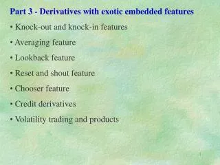
Part 3 - Derivatives with exotic embedded features Knock-out and knock-in features Averaging feature Lookback feature Reset and shout feature Chooser feature Credit derivatives Volatility trading and products. Path dependent feature. asset price. time. t 0. T.

E N D
Part 3 - Derivatives with exotic embedded features • Knock-out and knock-in features • Averaging feature • Lookback feature • Reset and shout feature • Chooser feature • Credit derivatives • Volatility trading and products
Path dependent feature asset price time t0 T The payoff of the option contract depends on the realization of the asset price within the whole life or part of the life of the option.
Most common types of path dependent options • Option is knocked out or activated when the asset price breaches some threshold value Barrier Options. • Average value of the asset prices over a certain period is • used as the strike Asian Options. • The strike price is determined by the realized maximum value of the asset price over a certain period Lookback Options.
The market for exotic options • Development of exotic products • increased flexibility for risk transfer and hedging • highly structured expression of expectation of asset • price movements • facilitation of trading in new risk dimension such as the • correlation between key financial variables • Modest volumes of trading and a relative lack of liquidity. These are associated with the difficulty in pricing, hedging / replicating (due to complex risk profiles).
asset price Knock-in and Knock-out up-barrier barrier level time knock-out Extinguished or activated upon achievement of relevant asset price level.
Features * barrier periods may cover only part of the option’s life * discretely monitored * can be in both European and American exercise format * barrier variable other than the underlying asset price * two-sided barriers (up-down) and sequential breaching * rebate may be paid upon knock out Advantage To achieve savings in premium; no need to pay for states believed to be unlikely to occur.
it is typically positive (for a call) but it becomes negative as it approaches the barrier delta: gamma: demonstrate very high gamma when the asset price is close to barrier usually higher than the non-barrier counterpart vega: pattern of time decay is not smooth, with sharp discontinuity when close to barrier theta:
Hedging difficulties circuit breaker effect upon knock out Market manipulation near barrier to trigger knock-out. “Soros (1995) knock-out options relate to ordinary options the way crack relates to cocaine.”
More complex versions of barrier options • The option could have two barrier levels (double barriers), one above the and below the current level of the index. The knockout condition then be (i) touching either one, or (ii) sequential breaching. • The barrier level could be based on another market (external barrier), say, the knock out of FTSE-100 option could be subject to the S&P 500 trading below a given level. • The barrier condition could exist for only part of the life time of the option (partial barriers). • Variable rather than a fixed barrier.
The second term then gives the price of the corresponding down-and-in call option. Down-and-out call option The call option is nullified when the asset price hits a down barrier B during the life of the option. The price formula for the continuously monitored down-and-out barrier call option is given by where cE(S, t) is the price of the vanilla counterpart.
Difficulties with dynamic hedging of barrier securities • 1. The underlying asset as the dynamic hedging instrument is • insensitive to changes in volatility. Option’s vega for • barrier securities is usually high. Vega risk is unhedgeable • except with other option-like securities. • Barrier options often have regions of high gamma, which • greatly increase the hedging error associated with dynamic • hedging.
Digital options(binary) • A pre-determined fixed payout if the option is at- or in-the-money (also called all-or-nothing, bet or lottery options). Primarily European in style. • Suited to markets where support and resistance levels are found, say, in the currency and bond markets. If an investor believes that a currency will not fall below a certain level, he can write a digital option to earn premium. • Writer faced with greater hedging challenges due to large gamma.
Note with embedded options Customer pays notional of 100 today. We pay a coupon of x% (p.a.) in 3 months. If spot price is above 100 at the end of the 3-month period, then the deal is terminated and we pay back 100 to him on that date. If the spot price is below 100, then a further coupon of 2% (p.a.) is paid in 6 months. The final redemption amount that the customer would obtain is given by Customer gets notional S/100 if S < 90 or S > 110, otherwise he would get back the notional.
The problem is to work out x%. The interesting thing is the barrier condition at the end of 3 months. The final payout for the customer can be decomposed into a combination of call option, put option and binary options.
Asian options Asian options are averaging options whose terminal payoff depends on some form of average. Arithmetic averaging = Geometric averaging = • Used by investors who are interested to hedge against the average price of a commodity over a period, rather than the end-of-the- period price e.g. Japanese exporters to the US, who are receiving stream of US dollar receipts over certain period, may use the Asian currency option to hedge the currency exposure. To minimize the impact of abnormal price fluctuation near expiration (avoid the price manipulation near expiration, in particular for thinly- traded commodities). •
Asian Averaging Options Average rate call: Average strike call: Uses Exposure as a future series of asset prices e.g. cost of production is sensitive to the prices of raw material. To prevent abnormal price manipulation on expiration date, arising perhaps from a lack of depth in the market.
Floating strike Asian call: Fixed strike Asian call: The option premium is expected to be lower than that of the vanilla options since the volatility of the average asset value should be lower than that of the terminal asset value; The delta and gamma tend to zero as time is approaching expiration. • • Set the strike to the average of prices over a period so as to avoid the exposure of market. The delta and gamma tend to that of the vanilla option with identical expiration data and strike equal to the average. • •
Shout options • The payoff upon shouting is another derivative with contractual specifications different from the original derivative. • The embedded shout feature in a call option allows its holder to lock in the profit via shouting while retaining the right to benefit from any future upside move in the payoff. • The terminal payoff of a shout call option is the form: • C = max(ST – K, L – K, 0), • where K is the strike price, ST is the terminal stock price and L is some ladder value installed at shouting. • The ladder value L is set to be the prevailing stock price St at the shouting instant t.
Shout feature • The terminal payoff is guaranteed to be at least St – K. • Obviously, the holder should shout only when St > K. • The number of shouting rights throughout the life of the contract may be more than one. • Some other restrictions may apply, say, the shouting instants are limited to some predetermined times.
Reset feature • This is the right given to the derivative holder to reset certain contract specifications in the original derivative. • Strike reset – strike reset to a lower strike for a call or to a higher strike for a put. • Maturity reset – extension of the maturity of a bond. • Constraints on reset • A limit to the magnitude of the strike adjustment. • Triggered by underlying price reaching certain level. • Reset allowed only on specific dates or limited period.
Example - Reset strike put option • The strike price is reset to the prevailing stock price upon shouting. • The shouting payoff is given by • max(St – ST, 0) = max(ST – K, St – K, 0) – (ST – K). • The shout call option can be replicated by the reset strike put and a forward contract • (put-call parity relation).
Example – Extendible bonds • Gives the holder the option of extending the term of the instrument, on or before a fixed date at a pre-determined coupon rate. • The 5.5 percent Government of Canada extendible bond was issued on October 1, 1959. It was exchangeable on or before June 1, 1962 into 5.5 percent bonds maturing October 1, 1975. • The three year initial bond was extendible into a 16 year bond at the holder’s option.
Example - S&P 500 index bear warrants with a three-month reset • Launched in the Chicago Board Options Exchange and the New York Stock Exchange (late 1996). • These warrants are index puts, where the strike price is automatically reset to the prevailing index value if the index value is higher than the original strike price on the reset date three months after the original issuance.
Lookback options Reset the strike to the realized lowest or highest market price during the lookback period. Payoff of the following forms: Partial lookbacks: selects a subset of the period from commencement to expiry as the lookback period. The premium increases with the length of the lookback period. Strike bonus rollover hedging strategy For the floating strike put, whenever a new maximum asset price is realized, replace the old put with a new put that has strike equal to the new maximum.
Uses of lookback options • Offshore debt or equity investments where the investor wishes to achieve the best currency over the relevant time period and wishes to uncouple the timing of the investment from the currency rate setting. • Perspectives of holder • Most advantageous if the realized volatility of the underlying asset price is higher that the implied volatility. • There will be a sharp move in the underlying asset price but is unsure when and for how long the price will move.
Questions:- Explain why the price of this callable option lies within the prices of the 1-year and 3-year non-callable counterparts. 1. 2. What is the impact of dividend yield on the optimal calling policy of this callable option? Callable Options Consider a 3-year call option with a fixed strike. After the first year and at every 6-month interval thereafter, the issuer has the right to call back the option. Upon calling, the holder is forced to exercise at the intrinsic value, or if the option is out-of-the-money, then the call option is terminated without any payment.
Range notes Provide investors with an above market coupon, but they must agree to forego coupon payments when LIBOR falls outside prescribed bounds. Example Suppose the market coupon for a conventional note is 6.5%. A range note pays 8.8% coupon semi-annually conditional on the 6-month LIBOR remains within 4.5-7.5%. The true coupon is computed on a daily accrual basis (coupons are counted on those dates when the LIBOR falls within the range).
Corridor risk • The investor loses coupon of rate 8.8% when LIBOR either exceeds 7.5% or below 4.5%. This is like the payoff of a digital cap and digital floor, respectively. This is called the “corridor risk”. • In essence, the investor shorts these two options in return for a higher coupon rate – selling volatility. • Investors have a strong view that rates will stay within a range and often they are structured to reflect an investor’s view that is contrary to a particular forward rate curve.
Example The Kingdom of Sweden issued dollar-denominated corridor Eurobonds in January 1994. The 200 million 2-year Sweden deal, for example, paid out Libor + 75 bp when the 3-month Libor fell between the following rates: 07/02/94 – 07/08/94; 3% to 4% 07/08/94 – 07/02/95; 3% to 4.75% 07/02/95 – 07/08/95; 3% to 5.50% 07/08/95 – 07/02/96; 3% to 6% The principal is fully protected, and the coupon is sacrificed only on days in which the 3-month Libor is outside the range.
Zero coupon accrual notes A hybrid version of a zero-coupon bond and an accrual note. • In a plain vanilla accrual note, an investor receives a coupon based on the number of days that a fixed income benchmark rate stays within a pre-specified range. • In a zero coupon bond, the investor knows at the time of purchase the bond’s maturity and effective yield. The zero coupon accrual note investor buys the note at a discount. Instead of a set maturity, there is a maximum maturity date. The note’s payout is capped at par. When the total return of the principal and the accrued coupon reaches par, the zero coupon accrual note matures.
Uses of zero coupon accrual notes In a rising interest rate environment, the maturity of the notes accelerates. Fixed income investors are thus able to reinvest their capital at the prevailing higher rates. • The inherent high convexity built into the zero coupon accrual notes benefits the buyer greatly by reducing the duration of the note as rates rise while lengthening duration as rates fall. • Unlike range notes where ranges are specified, this product allows investors to bet on a general move up in rates rather than the actual move in basis points.
Example of zero coupon accrual note A 3-year zero coupon accrual note linked to 6-month LIBOR sold at a price of 90 and a minimum annualized coupon of 2.5% (minimum coupon feature). • If the 6-month LIBOR does not rise substantially during the 3-year life of the note, the note will mature in 3 years.
Callable Range Accrual Note • The call options enable the investor to enhance his yield, compared to a standard Range Accrual Note. Even if the Note is called on the first call date, he would have benefited from a high coupon compared to the market conditions. • The Range Accrual structures are very popular with investors, especially when the implied volatility is high compared to the historical movements of the underlying index. • The Note will pay a higher coupon if, based on the forward curve, there is a high probability that the reference index will fix outside the range. The range can be tailored to match investor’s view on interest rates.
The graph below shows the forward distribution of the 6m Euribor as well as the upper barriers of the structure, and thus the probability for the index to fix within the range according to market conditions at the time of pricing.
credit risk interest rate risk FX risk volatility risk Risk de-aggregation Credit derivatives are over-the-counter contracts which allow the isolation and management of credit risk from all other components of risk. Off-balance sheet financial instruments that allow end users to buy and sell credit risk.
Product nature of credit derivatives Payoff depends on the occurrence of a credit event: • • default: any non-compliance with the exact specification of a contract • • price or yield change of a bond • • credit rating downgrade • In the case of the default of a bond, any loss in value from the default date until the • pricing date (a specified time period after the default date) becomes the value of • the underlying. • Credit derivatives can take the form of swaps or options. • In a credit swap, one party pays a fixed cashflow stream and the other party pays only if a credit event occurs (or payment based on yield spread). • A credit option would require the upfront premium and would pay off based on the occurrence of a credit event (or on a yield spread). • Pricing a credit derivative is not straightforward since modeling the • stochastic process driving the underlying’s credit risk is challenging.
Uses of credit derivatives To hedge against an increase in risk, or to gain exposure to a market with higher risk. • Creating customized exposure; e.g. gain exposure to Russian debts (rated below the manager’s criteria per her investment mandate). • Leveraging credit views - restructuring the risk/return profiles of credits. • Allow investors to eliminate credit risk from other risks in the investment instruments. Credit derivatives allow investors to take advantage of relative value opportunities by exploiting inefficiencies in the credit markets.
Credit spread derivatives • Options, forwards and swaps that are linked to credit spread. Credit spread = yield of debt – risk-free or reference yield • Investors gain protection from any degree of credit deterioration resulting from ratings downgrade, poor earnings etc. (This is unlike default swaps which provide protection against defaults and other clearly defined ‘credit events’.)
Credit spread option Use credit spread option to • hedge against rising credit spreads; • target the future purchase of assets at favorable prices. Example An investor wishing to buy a bond at a price below market can sell a credit spread option to target the purchase of that bond if the credit spread increases (earn the premium if spread narrows). at trade date, option premium counterparty investor if spread > strike spread at maturity Payout = notional (final spread – strike spread)+
Example The holder of the put has the right to sell the bond at the strike spread (say, spread = 330 bps) when the spread moves above the strike spread (corresponding to drop of bond price). May be used to target the future purchase of an asset at a favorable price. The investor intends to purchase the bond below current market price (300 bps above US Treasury) in the next year and has targeted a forward purchase price corresponding to a spread of 350 bps. She sells for 20 bps a one-year credit spread put struck at 330 bps to a counterparty (currently holding the bond and would like to protect the market price against spread above 330 bps). •spread < 330; investor earns the premium •spread > 330; investor acquires the bond at 350 bps
Several implied volatility values obtained simultaneously from different options (varying strikes and maturities) on the same underlying asset provide the market view about the volatility of the stochastic movement of the asset price. • Implied volatilities The only unobservable parameter in the Black-Scholes formulas is the volatility value, s. By inputting an estimated volatility value, we obtain the option price. Conversely, given the market price of an option, we can back out the corresponding Black-Scholes implied volatility.
Black wrote “It is rare that the value of an option comes out exactly equal to the price at which it trades on the exchange. There are several reasons for a difference between the value and price: (i) we may have the correct value; (ii) the option price may be out of line; (iii) we may have used the wrong inputs to the Black-Scholes formula; (iv) the Black-Scholes may be wrong. Normally, all reasons play a part in explaining a difference between value and price.” The market prices are correct (in the presence of sufficient liquidity) and one should build a model around the prices.
Different volatilities for different strike prices • Stock options – higher volatilities at lower strike and lower • volatilities at higher strikes • In a falling market, everyone needs out-of the-money puts • for insurance and will pay a higher price for the lower strike • options. • Equity fund managers are long billions of dollars worth of • stock and writing out-of-the-money call options against their • holdings as a way of generating extra income.
Commodity options – higher volatilities at higher strike and • lower volatilities at lower strikes • Government intervention – no worry about a large price fall. • Speculators are tempted to sell puts aggressively. • Risk of shortages – no upper limit on the price. Demand for • higher strike price options.
Volatility smiles Interest rate options – at-the-money option has a low volatility and either side the volatility is higher Propensity to sell at-the-money options and buy out-of- the-money options. For example, in the butterfly strategy, two at-the-money options are sold and one-out-of the-money option and one in-the-money option are bought.
Different volatilities across time • Supply and demand • When markets are very quiet, the implied volatilities of the near month • options are generally lower than those of the far month. When markets • are very volatile, the reverse is generally true. • In very volatile markets, everyone wants or needs to load with gamma. • Near-dated options provide the most gamma and the resultant buying • pressure will have the effect of pushing prices up. • In quiet markets no one wants a portfolio long of near dated options. • Use of a two-dimensional implied volatility matrix.
Floating volatilities As the stock price moves, the entire skewed profile also moves. This is because what was out-of-the-money option now becomes in-the-money option. Example If an investor is long a given option and believes that the market will price it at a lower volatility at a higher stock price then he may adjust the delta downwards (since the price appreciation is lower with a lower volatility).
Terminal asset price distribution as implied by market data probability In real markets, it is common that when the asset price is high, volatility tends to decrease, making it less probable for high asset price to be realized. When the asset price is low, volatility tends to increase, so it is more probable that the asset price plummets further down. S solid curve: distribution as implied by market data dotted curve: theoretical lognormal distribution
Extreme events in stock price movements Probability distributions of stock market returns have typically been estimated from historical time series. Unfortunately, common hypotheses may not capture the probability of extreme events, and the events of interest are rare and may not be present in the historical record. Examples On October 19, 1987, the two-month S & P 500 futures price fell 29%. Under the lognormal hypothesis of annualized volatility of 20%, this is a -27 standard deviation event with probability 10-160 (virtually impossible). 1. On October 13, 1989, the S & P 500 index fell about 6%, a -5 standard deviation event. Under the maintained hypothesis, this should occur only once in 14,756 years. 2.
X/S The market behavior of higher probability of large decline in stock index is better known to practitioners after Oct., 87 market crash. Implied volatility The market price of out-of-the-money call (puts) has become cheaper (more expensive) than the Black- Scholes theoretical price after the 1987 crash because of the thickening (thinning) of the left-end (right-end) tail of the terminal asset price distribution. • 1.0 A typical pattern of post-crash smile. The implied volatility drops against X/S.