Disjoint Sets
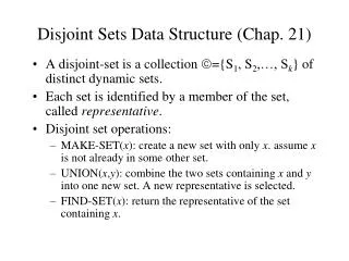
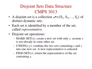
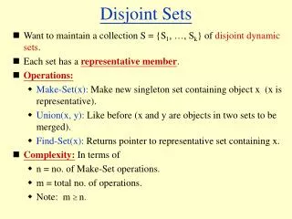
Disjoint Sets. Want to maintain a collection S = {S 1 , …, S k } of disjoint dynamic sets . Each set has a representative member . Operations: Make-Set(x): Make new singleton set containing object x (x is representative).

Disjoint Sets
E N D
Presentation Transcript
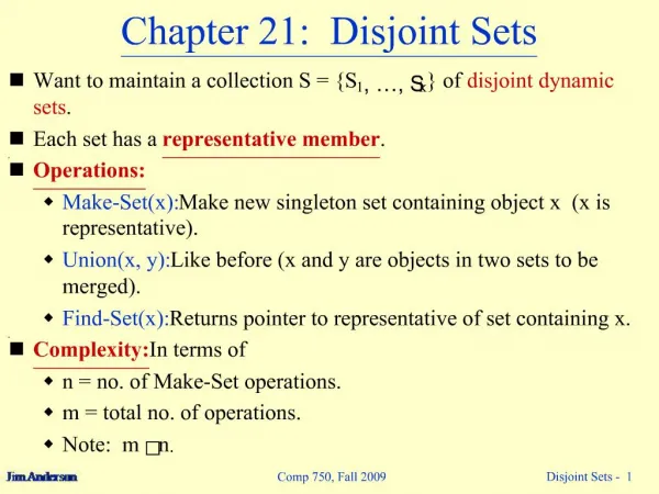
Disjoint Sets • Want to maintain a collection S = {S1, …, Sk} of disjoint dynamic sets. • Each set has a representative member. • Operations: • Make-Set(x): Make new singleton set containing object x (x is representative). • Union(x, y): Like before (x and y are objects in two sets to be merged). • Find-Set(x): Returns pointer to representative set containing x. • Complexity: In terms of • n = no. of Make-Set operations. • m = total no. of operations. • Note: m n.
Using Linked Lists Store set {a, b, c} as: a b c tail representative Make-Set and Find-Set are O(1). Union(x, y): Append x’s list onto the end of y’s list. Update representative pointers in x’s list. Time is linear in |x|. Running time for a sequence of m ops can take (m²) time. (Not very good.)
Example m = 2n – 1 operations. • Total Time is: • (n) = (m) for Make-Set ops. • for Union ops. • (m²) total. • (m) amortized. Operation M-S(x1) M-S(x2) M-S(xn) U(x1, x2) U(x2, x3) U(x3, x4) U(xn-1, xn) “Time” 1 1 1 1 2 3 n–1
Weighted-Union Heuristic • Keep track of list length in representative. • Modify Union so that smaller list is appended to longer one. • Time for Union is now proportional to the length of the smaller list.
Amortized Running Time of WUH Theorem 21.1: Sequence of m operations takes O(m + n lg n) time. Proof: M-S and F-S contribute O(m) total. What about Union? Time is dominated by no. of total times we change a rep. pointer. A given object’s rep. pointer can change at most lg n times.
Proof of Theorem 21.1 (Continued) • Note: n = no. of M-S’s = no. of objects • After object x’s rep. ptr. has been changed once, set has 2 members. • ……………………………………………twice..…….. 4 members. • ……………………………………………three times... 8 members. • ……………………………………………lg k times.. k members. • k n , so x’s rep. pointer can change at most lg n times. • O(n lg n) for n objects. • O(m + n lg n) total.
Disjoint-Set Forests a representative set is {a, b, c, d} b d M-S, F-S: Easy Union: As follows… c y x y x Union Will speed up sequence of Union, M-S, and F-S operations by means of two heuristics.
Two Heuristics • 1)Union by Rank • Store rank of tree in rep. • Rank tree size. • Make root with smaller rank point to root with larger rank. • 2)Path Compression • During Find-Set, “flatten” tree. d d c F-S(a) b a b c a
Operations • Make-Set(x) • p[x] := x; • rank[x] := 0 • Link(x, y) • if rank[x] > rank[y] then • p[y] := x • else • p[x] := y; • if rank[x] = rank[y] then • rank[y] := rank[y] + 1 • fi • fi • Find-Set(x) • if x p[x] then • p[x] := Find-Set(p[x]) • fi; • return p[x] • Union(x, y) • Link(Find-Set(x), Find-Set(y)) rank = u.b. on height
Find-Set c b a c a b F-S(a) p[a] := F-S(b) p[b] := F-S(c) { return c return c return c
Time Complexity • We cover the complexity analysis found in CLR rather than CLRS. • Note: This was Chapter 22 in CLR, which is why the remaining lemmas etc. are numbered the way they are. • Tight upper bound on time complexity: O(m (m,n)). • (m,n) = inverse of Ackermann’s function (almost a constant). • This bound, for a slightly different definition of than that given here, is shown in CLRS. • A slightly easier bound of O(m lg*n) is established in CLR.
Ackermann’s Function A(1, j) = 2j j 1 A(i,1) = A(i–1, 2) i 2 A(i, j) = A(i–1, A(i, j–1)) i, j 2 Grows very fast (inverse grows very slow). A(3, 4) = Notation: Note: This is one of several in-equivalent but similar definitions of Ackermann’s function found in the literature. CLRS gives a different definition. Please see the CLR handout. Powerpoint doesn’t do a great job with this notation.
Inverse of Ackermann’s Function • (m,n) = min{i1 : A(i, m/n) > lg n} • Note: Not a “true” mathematical inverse. • Intuition: Grows about as slowly as Ackermann’s function does fast. • How slowly? • Let m/n = k. • m n k 1. • We can show that A(i, k) A(i, 1) for all i 1. • Consider i = 4: • A(i, k) A(4, 1) = 1080 • So, (m,n) 4 if lg n < 1080, i.e., if n < 21080.
Bound We Establish • We establish O(m lg*n) as an upper bound. • Recall lg*n = min{i 0: lg(i) n 1}. • In particular: • And hence: lg*265536 = 5. • Thus, lg*n 5 for all practical purposes.
Example of Algorithm MS(a) ; MS(b) ; ... ; MS(i) ; MS(j) e/0 b/0 c/0 d/0 a/0 j/0 g/0 h/0 i/0 f/0 parent pointer rank U(a,b) ; U(c,d) ; U(e,f) ; U(g,h); U(i j) j/1 d/1 f/1 h/1 b/1 i/0 c/0 e/0 g/0 a/0
Example (Continued) j/1 d/1 f/1 h/1 b/1 i/0 c/0 e/0 g/0 a/0 U(a,d) d d/2 j/1 f/1 h/1 d b/1 d c/0 i/0 e/0 g/0 a/0 d
Example (Continued) d d/2 j/1 f/1 h/1 d b/1 d c/0 i/0 e/0 g/0 a/0 d U(f,h) d d/2 h h/2 j/1 d b/1 d c/0 f/1 h g/0 i/0 a/0 h e/0 h d
Example (Continued) d d/2 h h/2 j/1 d b/1 d c/0 f/1 h g/0 i/0 a/0 h e/0 h d U(d,h) h h/3 j/1 g/0 h d d/2 f/1 i/0 h b/1 d d c/0 e/0 h a/0 d
Example (Continued) h h/3 j/1 g/0 h d d/2 f/1 i/0 h b/1 d d c/0 e/0 h a/0 d U(e,j) h h/3 d/2 d e/0 f/1 g/0 j/1 b/1 d h h h c/0 d i/0 a/0 d
Example (Continued) h h/3 d/2 d e/0 f/1 g/0 j/1 b/1 d h h h c/0 d i/0 a/0 d FS(i) BC h h/3 Block 2 BC d/2 d Block 1 BC e/0 f/1 g/0 j/1 i/0 b/1 d Block 0 h h h c/0 PC d a/0 Block 0 d
Example (Continued) h h/3 d/2 d e/0 f/1 g/0 j/1 i/0 b/1 d h h h c/0 d a/0 d FS(a) h h/3 f/1 g/0 a/0 b/1 d/2 e/0 i/0 j/1 d h h h d d c/0 d
Properties of Ranks • Lemma 22.2: • (i) (x:: rank[x] rank[p[x]]). • (ii)(x: x p[x]: rank[x] < rank[p[x]]). • (iii) rank[x] is initially 0. • (iv) rank[x] does not decrease. • (v) Once x p[x] holds, rank[x] does not change. • (vi) rank[p[x]] is a monotonically increasing function of time. Proof: By induction on number of operations (see example).
Lemma 22.3 Lemma 22.3: For all tree roots x, size(x) 2rank[x]. no. of nodes in tree rooted at x Proof: Induction on number of Link operations Basis: Before first link, all ranks are 0 and each tree contains one node. Step: Consider Link(x,y). Assume lemma holds before this operation. We show it holds after. 2 cases.
Case 1: rank[x] rank[y] Assume rank[x] < rank[y]. y x y x Link(x,y) rank(y) size(y) rank(x) size(x) rank(y) size(y) rank(x) size(x) Note: rank(x) = rank(x) rank(y) = rank(y) size(y) = size(x) + size(y) 2rank(x) + 2rank(y) 2rank(y) = 2rank(y) No ranks or sizes change for any nodes other than y.
Case 2: rank[x] = rank[y] y x y x Link(x,y) rank(y) size(y) rank(x) size(x) rank(y) size(y) rank(x) size(x) Note: rank(x) = rank(x) rank(y) = rank(y) + 1 size(y) = size(x) + size(y) 2rank(x) + 2rank(y) 2rank(y) + 1 = 2rank(y)
Lemma 22.4 Lemma 22.4: For any integer r 0, there are at most n/2r nodes of rank r. • Proof: • Fix r. (r := 2 in example) • When rank r is assigned to some node x, label each node in the tree rooted at x by ‘x’. (See example.) • By Lemma 22.3, 2r nodes are labeled each time. • By Lemma 22.2, each node is labeled at most once, when its root is first assigned rank r. (See example.) • If there were more than n/2r nodes of rank r, then more than 2r (n/2r) = n nodes would be labeled by a node of rank r, a contradiction.
Corollary 22.5 Corollary 22.5: Every node has rank at most lg n. Proof: r > lg n n/ 2r < 1 nodes of rank r.
Proving the Time Bound Lemma 22.6: Suppose we convert a sequence S of m MS, U, and FS operations into a sequence S of m MS, Link, and FS operations by turning each Union into two FS operations followed by a Link. Then, if sequence S runs in O(m lg*n) time, sequence S runs in O(m lg*n) time. Only have to consider MS, Link, FS operations.
Theorem 22.7 Theorem 22.7: A sequence of m MS, L, and FS operations, n of which are MS operations, can be performed in worst-case time O(m lg*n). Proof: MS and Link take O(1) time. Key: Accurately charging FS. Partition ranks into blocks. Put rank r into block lg*r for r = 0, 1, ..., lg n. Corollary 22.5 Highest-numbered block is lg*(lg n) = lg*n – 1. –1 if j = –1 1 if j = 0 Define: B(j) 2 if j = 1 if j 2
Blocks For j = 0, 1, ... , lg*n – 1, Block j consists of the set of ranks {B( j–1 ) + 1, B( j–1 ) + 2, … , B( j )} B(–1) = –1 B(0) = 1 B(1) = 2 B(2) = 22 = 4 B(3) = B(4) = BlockRanks 0 0, 1 1 2 2 3, 4 3 5, … , 16 4 17, … , 65536
Charging for Find-Sets Two types of charges for FS:Block Charges and Path Charges. Consider FS(x0) x Charge each node as either Block Charge or Path Charge x1 x0 For j = 0, 1, ... , lg*n – 1, assess one block charge to the last node with rank in block j on the path x0, x1,...,x. Also assess one block charge to the child of the root, i.e., x -1. Assess other nodes in x0,... ,x a Path Charge. (See example.)
Claim Claim: Once a node other than a root or its child is assessed a B.C., it will never be assessed a P.C. Proof of Claim: rank[p[x]] – rank[x] is monotonically increasing. So, lg*(rank[p[x]]) – lg*(rank[x]) is monotonically increasing. Thus, once x and p[x] are in different blocks, they will always be in different blocks.
Remaining Goal Total cost of FS’s = Total B.C.’s + Total P.C.’s Want to show: Total B.C.’s + Total P.C.’s = O(m lg*n).
Bounding B.C.’s This part is easy. Block numbers range over 0, …, lg*n – 1 . lg*n + 1 B.C.’s per FS m FS’s total m (lg*n + 1) B.C.’s .
Bounding P.C.’s • Let N(j) = number of nodes whose ranks are in block j. • Claim: For all j 0, N(j) 3n / 2 B(j) . • Proof of Claim: • By Lemma 22.4, • For j = 0 : • N(0) n / 20 + n / 21 • = 3n / 2 • = 3n / 2B(0)
Proof of Claim (Continued) For j 1:
Bounding P.C.’s (Continued) Let P(n) overall number of path charges. P(n) (max number of nodes with ranks in Block j ) • (max number of path charges per node of Block j) Note: Any node in Block j that is assessed a P.C. will be in Block j after all m operations. By claim, upper-bounded by 3n/ 2B(j) If node x is assessed a P.C. : rank > r Path Compression x … … rank r x x gets new parent with increased rank
Bounding P.C.’s (Continued) So, every time x is assessed a P.C., it gets a new parent with increased rank. Note: x’s rank is not changed by Path Compression. Suppose x has a rank in Block j. Repeated P.C.’s to x will ultimately result in x’s parent having a rank in a Block higher than j. From that point onward, x is assessed B.C.’s, not P.C.’s. Worst Case: x has lowest rank in Block j, i.e., B(j–1) + 1, and x’s parents’ ranks successively take on the values B(j–1) + 2, B(j–1) + 3, …, B(j).
Finally! Hence, x can be assesses at most B(j) – B( j – 1 ) – 1 P.C.’s. Therefore, Thus, FS operations contribute: O(m(lg*n + 1) + n lg*n) = O(m lg*n). MS and Link contribute O(n). Entire sequence takes O(m lg*n).