Memory Management Techniques - Chapter 8
This chapter provides a detailed description of various memory hardware organization methods and memory management techniques, such as paging and segmentation. It also discusses the Intel Pentium architecture and its support for different memory management approaches.

Memory Management Techniques - Chapter 8
E N D
Presentation Transcript
Chapter 8: Memory Management • Background • Swapping • Contiguous Memory Allocation • Segmentation • Paging • Structure of the Page Table • Example: The Intel 32 and 64-bit Architectures • Example: ARM Architecture
Objectives • To provide a detailed description of various ways of organizing memory hardware • To discuss various memory-management techniques, including paging and segmentation • To provide a detailed description of the Intel Pentium, which supports both pure segmentation and segmentation with paging
Background • Program must be brought (from disk) into memory and placed within a process for it to be run • Main memory and registers are only storage CPU can access directly • Memory unit only sees a stream of addresses + read requests, or address + data and write requests • Register access in one CPU clock (or less) • Main memory can take many cycles, causing a stall • Cachesits between main memory and CPU registers • Protection of memory required to ensure correct operation
Base and Limit Registers • To make sure that each process has a separate memory space. A pair of baseandlimitregisters define the logical address space for user process. • CPU must check every memory access generated in user mode to be sure it is between base and limit for that user Any attempt by a program executing in user mode to access operating-system memory or other users’ memory results in a trap to the operating system, which treats the attempt as a fatal error
Address Binding • The processes on the disk that are waiting to be brought into memory for execution form the input queue. • The normal procedure is to select one of the processes in the input queue and to load that process into memory. when the process terminates its memory space is declared available. • Further, addresses represented in different ways at different stages of a program’s life • Source code addresses usually symbolic • Compiled code addresses bind to relocatable addresses • i.e. “14 bytes from beginning of this module” • Linker or loader will bind relocatable addresses to absolute addresses • i.e. 74014 • Each binding maps one address space to another
Binding of Instructions and Data to Memory • Address binding of instructions and data to memory addresses can happen at three different stages • Compile time: If you know at compile time where the process will reside in memory, then, absolute codecan be generated; If, at some later time, the starting location changes, then it will be necessary to recompile this code. • Load time: If it is not known at compile time where the process will reside in memory, then the compiler must generate relocatable code. In this case, final binding is delayed until load time. If the starting address changes, we need only reload the user code to incorporate this changed value. • Execution time: If the process can be moved during its execution from one memory segment to another, then binding must be delayed until run time
Logical vs. Physical Address Space • An address generated by the CPU is commonly referred to as a logical address, also referred to as virtual address • Whereas an address seen by the memory unit— that is, the one loaded into the memory-address register of the memory—is commonly referred to as a physical address. • The compile-time and load-time address-binding methods generate identical logical and physical addresses. • However, the execution-time address binding scheme results in differing logical and physical addresses. • Logical address space is the set of all logical addresses generated by a program • Physical address space is the set of all physical addresses generated by a program
Memory-Management Unit (MMU) • The run-time mapping from virtual to physical addresses is done by a hardware device called the memory-management unit (MMU). • To start, consider simple scheme where the value in the relocation register (base register) is added to every address generated by a user process at the time it is sent to memory • For example, if the base (relocation register ) is at 14000, then an attempt by the user to address location 0 is dynamically relocated to location 14000; an access to location 346 is mapped to location 14346. • The user program deals with logical addresses; it never sees the real physical addresses • The user program generates only logical addresses and thinks that the process runs in locations 0 to max. • However, these logical addresses must be mapped to physical addresses before they are used.
Swapping • A process can be swapped temporarily out of memory to a backing store, and then brought back into memory for continued execution • Total physical memory space of processes can exceed physical memory • Backing store– fast disk large enough to accommodate copies of all memory images for all users • Roll out, roll in– swapping variant used for priority-based scheduling algorithms; lower-priority process is swapped out so higher-priority process can be loaded and executed • Major part of swap time is transfer time;
Context Switch Time including Swapping • The context-switch time in such a swapping system is fairly high. • To get an idea of the context-switch time, • let’s assume that the user process is 100 MB in size and the backing store is a standard hard disk with a transfer rate of 50 MB per second. • The actual transfer of the 100-MB process to or from main memory takes • 100 MB/50 MB per second = 2 seconds • Since we must both swap out and swap in, the total swap time is 4 seconds
Contiguous Allocation • Main memory must support both OS and user processes • Limited resource, must allocate efficiently • Main memory usually into two partitions: • Resident operating system, usually held in low memory and user processes then held in high memory • We usually want several user processes to reside in memory at the same time. We therefore need to consider how to allocate available memory to the processes that are waiting to be brought into memory. • In contiguous memory allocation, each process is contained in a single contiguous section of memory.
Contiguous Allocation (Cont.) • Relocation registers used to protect user processes from each other, and from changing operating-system code and data • Base register contains value of smallest physical address • Limit register contains range of logical addresses – each logical address must be less than the limit register • MMU maps logical address dynamically by adding the value in the relocation register. This mapped address is sent to memory.
Multiple-partition allocation • Multiple-partition allocation:fixed-sizedpartitions scheme • divide memory into several fixed-sizedpartitions. Each partition may contain exactly one process. • Thus, the degree of multiprogramming is bound by the number of partitions. • when a partition is free, a process is selected from the input queue and is loaded into the free partition. • When the process terminates, the partition becomes available for another process. • Multiple-partition allocation:variable-partition scheme • In the variable-partition scheme, the operating system keeps a table indicating which parts of memory are available and which are occupied. • Initially, all memory is available for user processes and is considered one large block of available memory • Hole – block of available memory; holes of various size are scattered throughout memory • When a process arrives, it is allocated memory from a hole large enough to accommodate it. When a process terminates, it releases its memory partition, adjacent free partitions combined
Dynamic Storage-Allocation Problem How to satisfy a request of size n from a list of free holes? • First-fit: Allocate the first hole that is big enough • Best-fit: Allocate the smallest hole that is big enough; must search entire list, unless ordered by size • Produces the smallest leftover hole • Worst-fit: Allocate the largest hole; must also search entire list • Produces the largest leftover hole First-fit and best-fit better than worst-fit in terms of speed and storage utilization
Fragmentation • External Fragmentation– total memory space exists to satisfy a request to load a process, but it is not contiguous • First fit analysis reveals that given N blocks allocated, 0.5 N blocks lost to fragmentation • 1/3 may be unusable -> 50-percent rule • Internal Fragmentation– allocated memory may be slightly larger than requested memory; this size difference is memory internal to a partition, but not being used
Fragmentation (Cont.) • Reduce external fragmentation by compaction • Shuffle memory contents to place all free memory together in one large block • Compaction is possible only if relocation is dynamic, and is done at execution time • The simplest compaction algorithm is to move all processes toward one end of memory; all holes move in the other direction, producing one large hole of available memory • Another possible solution to the external-fragmentation problem is to permit the logical address space of the processes to be noncontiguous, thus allowing a process to be allocated physical memory wherever such memory is available. • Two techniques achieve this solution: segmentation and paging
Segmentation • Memory-management scheme that supports user view of memory • A program is a collection of segments • A segment is a logical unit such as: main program, procedure, function, method, object, local variables, global variables, common block, stack, symbol table, arrays • Each segment has a name and a length. • Elements within a segment are identified by their offset from the beginning of the segment: • Ex: The first statement of the main program
1 4 2 3 Logical View of Segmentation 1 2 3 4 user space physical memory space
Segmentation Architecture • For simplicity of implementation, segments are numbered and are referred to by a segment number, rather than by a segment name. • Logical address consists of a two tuple: <segment-number, offset>, • Segment table– map two-dimensional user-defined addresses into one-dimensional physical addresses; • each table entry has: • segment base– contains the starting physical address where the segments reside in memory • segmentlimit– specifies the length of the segment • Segment-table base register (STBR)points to the segment table’s location in memory • Segment-table length register (STLR)indicates number of segments used by a program; segment number s is legal if s < STLR
Segmentation Hardware A logical address consists of two parts: a segment number, s, and an offset , d. The segment number is used as an index to the segment table. The offset d of the logical address must be between 0 and the segment limit. If it is not, error When an offset is legal, it is added to the segment base to produce the address in physical memory of the desired byte.
EX: Store the following segments in physical memory and show physical address space for each segment.
Paging • Paging is a memory-management scheme that permits the physical address space of a process to be noncontiguous. • Paging avoids external fragmentation and the need for compaction. • The basic method for implementing paging • Divide physical memory into fixed-sized blocks called frames • Size is power of 2, between 512 bytes and 16 Mbytes • Divide logical memory into blocks of same size called pages • Keep track of all free frames • To run a program of size Npages, need to find N free frames and load program from back store to physical main memory • Set up a page table to translate logical to physical addresses • The backing store is divided into fixed-sized blocks that are of the same size as the memory frames • Still have Internal fragmentation
Address Translation Scheme • Address generated by CPU is divided into: • Page number (p)– used as an index into a page table which contains base address of each page in physical memory • Page offset (d)– combined with base address to define the physical memory address that is sent to the memory unit • For given logical address space 2m and page size2n
Paging Example • consider the memory in Figure 8.9. • Using a page size of 4 bytes and a physical memory of 32 bytes (8 pages), • For given logical address space 2m a= 16 and page size2n= 4 n= 2 and m = 4. • we show how the user’s view of memory can be mapped into physical memory. • First byte physical address of frame number x = x * frame size. • Logical address 0 is page 0, offset 0. Indexing into the page table, we find that page 0 is in frame 5. Thus, logical address 0 maps to physical address 20 [= (5 × 4) + 0]. • Logical address 3 (page 0, offset 3) maps to physical address 23 [= (5 × 4) + 3]. • Logical address 4 is page 1, offset 0; according to the page table, page 1 is mapped to frame 6. • Thus, logical address 4 maps to physical address 24 [= (6 × 4) + 0]. Logical address 13 maps to physical address 9.
Paging Example n=2 and m=4 32-byte memory and 4-byte pages
Paging (Cont.) • Calculating internal fragmentation • Page size = 2,048 bytes • Process size = 72,766 bytes • 35 pages + 1,086 bytes • Internal fragmentation of 2,048 - 1,086 = 962 bytes • Worst case fragmentation = 1 frame – 1 byte • On average fragmentation = 1 / 2 frame size
Free Frames When a process arrives in the system to be executed, its size, expressed in pages. Each page of the process needs one frame. Thus, if the process requires n pages, at least n frames must be available in memory. If n frames are available, they are allocated to this arriving process. The first page of the process is loaded into one of the allocated frames, and the frame number Before allocation After allocation
Implementation of Page Table • Page table is kept in main memory • Page-table base register (PTBR)points to the page table • Page-table length register (PTLR)indicates size of the page table • In this scheme every data/instruction access requires two memory accesses • One for the page table and one for the data / instruction • The standard solution to this problem is to use a special, small, fast lookup hardware cache, called a translation look-aside buffer (TLB).
Translation Look-aside Buffer (TLB). • The TLB is associative, high-speed memory. • Each entry in the TLB consists of two parts: • a key (or tag) and a value. • When the associative memory is presented with an item, the item is compared with all keys simultaneously. • If the item is found, the corresponding value field is returned. • The search is fast; the hardware, however, is expensive. • Typically, the number of entries in a TLB is small,
Translation Look-aside Buffer (TLB). • The TLB is used with page tables in the following way. • The TLB contains only a few of the page-table entries. • When a logical address is generated by the CPU, its page number is presented to the TLB. • If the page number is found, its frame number is immediately available and is used to access memory. • If the page number is not in the TLB (known as a TLB miss), a memory reference to the page table must be made. • When the frame number is obtained, we can use it to access memory. In addition, we add the page number and frame number to the TLB, so that they will be found quickly on the next reference. • If the TLB is already full of entries, the operating system must select one for replacement
TLB Hit ratio and Miss ratio • The percentage of times that a particular page number is found in the TLB is called the hit ratio. • An 80-percent hit ratio, for example, means that we find the desired page number in the TLB 80 percent of the time. • If it takes 20 nanoseconds to search the TLB and 100 nanoseconds to access memory, then a mapped-memory access takes 120 nanoseconds when the page number is in the TLB. • If we fail to find the page number in the TLB (20 nanoseconds), then we must first access memory for the page table and frame number (100 nanoseconds) and then access the desired byte in memory (100 nanoseconds), for a total of 220 nanoseconds. • To find the effective memory-access time, we weight the case by its probability: • effective access time= hit ratio X (TLB access time + memory access time) + miss ratio X (TLB access time +2* memory access time ) • effective access time = 0.80 × 120 + 0.20 × 220 = 140 nanoseconds. • For a 98-percent hit ratio, we have effective access time = 0.98 × 120 + 0.02 × 220 = 122 nanoseconds.
Shared Pages • Shared code • One copy of read-only code shared among processes (i.e., text editors, compilers, window systems) • Similar to multiple threads sharing the same process space • Also useful for interprocess communication if sharing of read-write pages is allowed • Private code and data • Each process keeps a separate copy of the code and data • The pages for the private code and data can appear anywhere in the logical address space
Shared Pages Example Here we see a three-page editor—each page 50 KB in size—being shared among three processes. • Only one copy of the editor need be kept in physical memory. • Each user’s page table maps onto the same physical copy of the editor, but data pages are mapped onto different frames. • Thus, to support 40 users, we need only one copy of the editor (150 KB), plus 40 copies of the 50 KB of data space per user. • The total space required is now 2,150 KB instead of 8,000 KB if no shared pages is used.