Download

1 / 77
780 likes | 972 Vues
Last lecture. Passive Stereo Spacetime Stereo. Today. Structure from Motion: Given pixel correspondences, how to compute 3D structure and camera motion?. Slides stolen from Prof Yungyu Chuang. Epipolar geometry & fundamental matrix. The epipolar geometry.

E N D
Last lecture • Passive Stereo • Spacetime Stereo
Today • Structure from Motion: Given pixel correspondences, how to compute 3D structure and camera motion? Slides stolen from Prof Yungyu Chuang
The epipolar geometry What if only C,C’,x are known?
The epipolar geometry C,C’,x,x’ and X are coplanar epipolar geometry demo
The epipolar geometry All points on project on l and l’
The epipolar geometry Family of planes and lines l and l’ intersect at e and e’
The epipolar geometry epipolar plane = plane containing baseline epipolar line = intersection of epipolar plane with image epipolar pole = intersection of baseline with image plane = projection of projection center in other image epipolar geometry demo
p p’ T=C’-C The equation of the epipolar plane through X is The fundamental matrix F R C’ C
essential matrix The fundamental matrix F
p p’ T=C’-C The fundamental matrix F R C’ C
Let M and M’ be the intrinsic matrices, then fundamental matrix The fundamental matrix F
p p’ T=C’-C The fundamental matrix F R C’ C
The fundamental matrix F • The fundamental matrix is the algebraic representation of epipolar geometry • The fundamental matrix satisfies the condition that for any pair of corresponding points x↔x’ in the two images
The fundamental matrix F F is the unique 3x3 rank 2 matrix that satisfies x’TFx=0 for all x↔x’ • Transpose: if F is fundamental matrix for (P,P’), then FT is fundamental matrix for (P’,P) • Epipolar lines: l’=Fx & l=FTx’ • Epipoles: on all epipolar lines, thus e’TFx=0, x e’TF=0, similarly Fe=0 • F has 7 d.o.f. , i.e. 3x3-1(homogeneous)-1(rank2) • F maps from a point x to a line l’=Fx (not invertible)
The fundamental matrix F • It can be used for • Simplifies matching • Allows to detect wrong matches
Estimation of F — 8-point algorithm • The fundamental matrix F is defined by for any pair of matches x and x’ in two images. • Let x=(u,v,1)T and x’=(u’,v’,1)T, each match gives a linear equation
8-point algorithm • In reality, instead of solving , we seek f to minimize , least eigenvector of .
8-point algorithm • To enforce that F is of rank 2, F is replaced by F’ that minimizes subject to . • It is achieved by SVD. Let , where • , let • then is the solution.
8-point algorithm % Build the constraint matrix A = [x2(1,:)‘.*x1(1,:)' x2(1,:)'.*x1(2,:)' x2(1,:)' ... x2(2,:)'.*x1(1,:)' x2(2,:)'.*x1(2,:)' x2(2,:)' ... x1(1,:)' x1(2,:)' ones(npts,1) ]; [U,D,V] = svd(A); % Extract fundamental matrix from the column of V % corresponding to the smallest singular value. F = reshape(V(:,9),3,3)'; % Enforce rank2 constraint [U,D,V] = svd(F); F = U*diag([D(1,1) D(2,2) 0])*V';
8-point algorithm • Pros: it is linear, easy to implement and fast • Cons: susceptible to noise
! Problem with 8-point algorithm ~100 ~10000 ~100 ~10000 ~10000 ~100 ~100 1 ~10000 Orders of magnitude difference between column of data matrix least-squares yields poor results
Normalized 8-point algorithm normalized least squares yields good results Transform image to ~[-1,1]x[-1,1] (0,500) (700,500) (-1,1) (1,1) (0,0) (0,0) (700,0) (-1,-1) (1,-1)
Normalized 8-point algorithm • Transform input by , • Call 8-point on to obtain
Normalized 8-point algorithm A = [x2(1,:)‘.*x1(1,:)' x2(1,:)'.*x1(2,:)' x2(1,:)' ... x2(2,:)'.*x1(1,:)' x2(2,:)'.*x1(2,:)' x2(2,:)' ... x1(1,:)' x1(2,:)' ones(npts,1) ]; [U,D,V] = svd(A); F = reshape(V(:,9),3,3)'; [U,D,V] = svd(F); F = U*diag([D(1,1) D(2,2) 0])*V'; [x1, T1] = normalise2dpts(x1); [x2, T2] = normalise2dpts(x2); % Denormalise F = T2'*F*T1;
Normalization function [newpts, T] = normalise2dpts(pts) c = mean(pts(1:2,:)')'; % Centroid newp(1,:) = pts(1,:)-c(1); % Shift origin to centroid. newp(2,:) = pts(2,:)-c(2); meandist = mean(sqrt(newp(1,:).^2 + newp(2,:).^2)); scale = sqrt(2)/meandist; T = [scale 0 -scale*c(1) 0 scale -scale*c(2) 0 0 1 ]; newpts = T*pts;
RANSAC repeat select minimal sample (8 matches) compute solution(s) for F determine inliers until (#inliers,#samples)>95% or too many times compute F based on all inliers
From F to R, T If we know camera parameters Hartley and Zisserman, Multiple View Geometry, 2nd edition, pp 259
Main trick • Prewarp with a homography to rectify images • So that the two views are parallel • Because linear interpolation works when views are parallel
Problem with morphing • Without rectification
morph morph prewarp prewarp output input input homographies
Triangulation • Problem: Given some points in correspondence across two or more images (taken from calibrated cameras), {(uj,vj)}, compute the 3D location X CSE 576 (Spring 2005): Computer Vision
Triangulation • Method I: intersect viewing rays in 3D, minimize: • X is the unknown 3D point • Cj is the optical center of camera j • Vj is the viewing ray for pixel (uj,vj) • sj is unknown distance along Vj • Advantage: geometrically intuitive X Vj Cj CSE 576 (Spring 2005): Computer Vision
Triangulation • Method II: solve linear equations in X • advantage: very simple • Method III: non-linear minimization • advantage: most accurate (image plane error) CSE 576 (Spring 2005): Computer Vision
Structure from motion structure from motion: automatic recovery of camera motion and scene structure from two or more images. It is a self calibration technique and called automatic camera tracking or matchmoving. Unknown camera viewpoints
Applications • For computer vision, multiple-view shape reconstruction, novel view synthesis and autonomous vehicle navigation. • For film production, seamless insertion of CGI into live-action backgrounds
Structure from motion geometry fitting 2D feature tracking 3D estimation optimization (bundle adjust) SFM pipeline
Structure from motion • Step 1: Track Features • Detect good features, Shi & Tomasi, SIFT • Find correspondences between frames • Lucas & Kanade-style motion estimation • window-based correlation • SIFT matching
Structure from Motion • Step 2: Estimate Motion and Structure • Simplified projection model, e.g., [Tomasi 92] • 2 or 3 views at a time [Hartley 00]
Structure from Motion • Step 3: Refine estimates • “Bundle adjustment” in photogrammetry • Other iterative methods
Structure from Motion • Step 4: Recover surfaces (image-based triangulation, silhouettes, stereo…) Good mesh