Download

1 / 16
160 likes | 185 Vues
Utilize case-control study data for esophageal cancer, correcting miscoded values and outliers. Perform logistic regression modeling for binary and ordinal outcomes using SAS. Interpret log odds and odds ratio for alcohol consumption predictors.

E N D
Labs 6 & 7 Case-Control Analysis ----Logistic Regression Henian Chen, M.D., Ph.D. Applied Epidemiologic Analysis - P8400 Fall 2002
Data Files Today we will use the case-control study data of esophageal cancer. If you use “infile” statement to read the ‘case-control978. dat’ file,Please make sure that you corrected the miscoded values and the two abnormally high values for alcohol. I corrected case-control978.dbf, case-control978.wk3, and case-control978.txt. You are welcome to use one of them. procimport datafile='a:case-control978.txt' out=case_control978 dbms=tab replace; getnames=yes; run; procimport datafile='a:case-control978.wk3' out= case_control978 dbms=wk3 replace; getnames=yes; run; procimport datafile='a:case-control978.dbf' out= case_control978 dbms=dbf replace; run; Applied Epidemiologic Analysis - P8400 Fall 2002
Logistic Regression Model A regression model in which the dependent variable is binary (yes, no). A form of the generalized linear model in which the link function is the logit, and the regression parameters are expressed as log odds associated with unit increase in the predictors. For ordinal response outcomes (no pain, slight pain, substantial pain), we can model the cumulative logits by performing ordered logistic regression using the proportional odds model For nominal outcomes (Democrate, Republicans, Independents), we can model the generalized logits by performing logistic analysis using the log-linear model Applied Epidemiologic Analysis - P8400 Fall 2002
Logistic Regression for Intercept only SAS Program proclogisticdata=case_control978 descending; model status=; run; * Descending: to get the probability and OR for dependent variable=1 SAS Output The LOGISTIC Procedure Model Information Data Set WORK.CASE_CONTROL978 Response Variable status Number of Response Levels 2 Number of Observations 978 Model binary logit Optimization Technique Fisher's scoring Applied Epidemiologic Analysis - P8400 Fall 2002
Logistic Regression for Intercept only SAS Output Response Profile Ordered Total Value status Frequency 1 1 200 2 0 778 Probability modeled is status=1. Model Convergence Status Convergence criterion (GCONV=1E-8) satisfied. -2 Log L = 990.8635 Analysis of Maximum Likelihood Estimates Standard Wald Parameter DF Estimate Error Chi-Square Pr > ChiSq Intercept 1 -1.3584 0.0793 293.5837 <.0001 Applied Epidemiologic Analysis - P8400 Fall 2002
Logistic Regression for Intercept only 1. Calculate the log odds In our model, intercept (α) = -1.3584, -1.3584 is the log odds of cancer for total sample 2. Take the antilog to get the odds Odds=exp(-1.3584)=0.2571 3. Divide the odds by (1+odds) to get the P (P means probability in cohort or population, in case-control study P means proportion) P = 0.2571/(1+0.2571)=0.2045 = 200/(200+778) P is related to α in Logistic Model Applied Epidemiologic Analysis - P8400 Fall 2002
Logistic Regression for Dichotomous Predictor Alcohol Consumption (alcgrp): 0=0-39 gm/day; 1=40+ gm/day SAS Program proclogisticdata=case_control978 descending; model status=alcgrp; run; SAS Output Model Fit Statistics Criterion Intercept Only Intercept and Covariates -2 Log L 990.863 901.036 Likelihood Ratio Test G = 990.863 – 901.036 = 89.827 df = 1 The model with variable ‘alcgrp’ is significantly. Applied Epidemiologic Analysis - P8400 Fall 2002
Logistic Regression for Dichotomous Predictor SAS Output Analysis of Maximum Likelihood Estimates Standard Wald Parameter DF Estimate Error Chi-Square Pr > ChiSq Intercept 1 -2.5911 0.1925 181.1314 <.0001 alcgrp 1 1.7641 0.2132 68.4372 <.0001 Odds Ratio Estimates Point 95% Wald Effect Estimate Confidence Limits alcgrp 5.836 3.843 8.864 OR = exp(β) = exp(1.7641) = 5.836 Heavy drinkers (alcgrp=1) are about 6 times more likely to get cancer than light drinkers (alcgrp=0). OR is not related to α in Logistic Model Applied Epidemiologic Analysis - P8400 Fall 2002
Logistic Regression for Dichotomous Predictor 1. Calculate the log odds Light drinkers (alcgrp=0), log odds=-2.5911 Heavy drinkers (alcgrp=1), log odds=-2.5911+1.7641=-0.827 2. Take the antilog to get the odds Light drinkers, Odds=exp(-2.5911)=0.0749 Heavy drinkers, Odds=exp(-0.827)=0.4374 3. Divide the odds by (1+odds) to get the P(x) Light drinkers, P(x)=0.0749/(1+0.0749)=0.0697 Heavy drinkers, P(x)=0.4374/(1+0.4374)=0.3043 Applied Epidemiologic Analysis - P8400 Fall 2002
Logistic Regression for Ordinal Predictor Alcohol Consumption (alcgrp4): 0=0-39 gm/day; 1=40-79 gm/day 2=80-119 gm/day; 3=120+ gm/day SAS Program proclogisticdata=case_control978 descending; model status=alcgrp4; run; SAS Output Model Fit Statistics Criterion Intercept Only Intercept and Covariates -2 Log L 990.863 846.467 Likelihood Ratio Test G = 990.863 – 846.467 = 144.396 df = 1 The model with variable ‘alcgrp4’ is significantly. Applied Epidemiologic Analysis - P8400 Fall 2002
Logistic Regression for Ordinal Predictor SAS Output Analysis of Maximum Likelihood Estimates Standard Wald Parameter DF Estimate Error Chi-Square Pr > ChiSq Intercept 1 -2.4866 0.1459 290.4172 <.0001 alcgrp4 1 1.0453 0.0934 125.2007 <.0001 Odds Ratio Estimates Point 95% Wald Effect Estimate Confidence Limits alcgrp4 2.844 2.368 3.416 OR = exp(1.0453) = 2.844. Men with alcgrp4=1 are about 3 times more likely to get cancer than men with alcgrp4=0. This OR is also for alcgrp4= 1 vs. alcgrp4=2; or alcgrp4=2 vs. alcgrp4=3. OR = exp[(3-1)*1.0453] = exp(2.0906) = 8.090 for alcgrp4=1 vs. alcgrp4=3 OR = exp[(3-0)*1.0453] = exp(3.1359) = 23.009 for alcgrp4=0 vs. alcgrp4=3 Applied Epidemiologic Analysis - P8400 Fall 2002
OR=exp(βx) is a special case when 1. X is a binary variable 2. No interactions between X and other variables If X is not a binary variable OR=exp[βx(X*-X**)] If X is not a binary variable, and there is a interaction between X and W, OR=exp[(X*-X**)(βx+ βxwW)] Applied Epidemiologic Analysis - P8400 Fall 2002
Logistic Regression for Continuous Predictor Alcohol Consumption (alcohol): daily consumption in grams SAS Program proclogisticdata=case_control978 descending; model status=alcohol; run; SAS Output Analysis of Maximum Likelihood Estimates Standard Wald Parameter DF Estimate Error Chi-Square Pr > ChiSq Intercept 1 -2.9741 0.1807 270.9266 <.0001 alcohol 1 0.0261 0.00232 126.4179 <.0001 Odds Ratio Estimates Point 95% Wald Effect Estimate Confidence Limits alcohol 1.026 1.022 1.031 Applied Epidemiologic Analysis - P8400 Fall 2002
Logistic Regression for Continuous Predictor OR = exp(0.0261) = 1.026. The odds of cancer increase by a factor of 1.026 for each unit in alcohol consumption OR = exp[40*(0.0261)] = exp(1.044) = 2.8406 for a 40-grams increase in alcohol consumption per day OR = exp[120*(0.0261)] = 22.825 for a man who drinks 160 grams per day compare with a man who is similar in other respects but drinks 40 grams per day. Applied Epidemiologic Analysis - P8400 Fall 2002
Interaction in Logistic Regression model status = α + β1 alcgrp + β2 tobgrp β1 : the effect of alcohol on cancer, controlling for tobacco (i.e., the same OR across levels of tobacco) β2 :the effect of tobacco on cancer, controlling for alcohol (i.e., the same OR across levels of alcohol) model status = α + β1 alcgrp + β2 tobgrp + β3 alcgrp*tobgrp β1 : the effect of alcohol on cancer among non-smokers (tobgrp=0) β2 :the effect of tobacco on cancer among non-drinkers (alcgrp=0) β3 : interaction between smokers and drinkers Applied Epidemiologic Analysis - P8400 Fall 2002
Interaction in Logistic Regression model status = -3.33 + 2.28 (alcgrp) + 1.38 (tobgrp) –0.98 (alcgrp*tobgrp) Log odds odds A: alcgrp=0 & tobgrp=0 2.28*0 + 1.38*0 – 0.98*0*0 = 0.00 1.00 B: alcgrp=1 & tobgrp=0 2.28*1 + 1.38*0 – 0.98*1*0 = 2.28 9.78 C: alcgrp=0 & tobgrp=1 2.28*0 + 1.38*1 – 0.98*0*1 = 1.38 3.97 D: alcgrp=1 & tobgrp=1 2.28*1 + 1.38*1 – 0.98*1*1 = 2.68 14.59 Odds Ratio A vs. B 9.78 = 9.78/1.00 A vs. C 3.97 = 3.97/1.00 A vs. D 14.59 = 14.59/1.00 B vs. D 1.49 = 14.59/9.78 C vs. D 3.68 = 14.59/3.97 Applied Epidemiologic Analysis - P8400 Fall 2002