Download
1 / 1
20 likes | 166 Vues
A new car following model: comprehensive optimal velocity model Jun fang Tian , Bin jia , Xin gang Li MOE Key Laboratory for Urban Transportation Complex Systems Theory and Technology, Beijing Jiaotong University, Beijing 100044, P.R.China E-mail: bjia@bjtu.edu.cn. Contributions. Results.

E N D
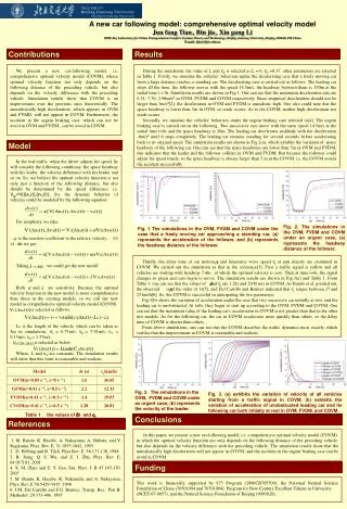
A new car following model: comprehensive optimal velocity model Jun fang Tian, Bin jia, Xin gang Li MOE Key Laboratory for Urban Transportation Complex Systems Theory and Technology, Beijing Jiaotong University, Beijing 100044, P.R.China E-mail: bjia@bjtu.edu.cn Contributions Results We present a new car-following model, i.e. comprehensive optimal velocity model (COVM), whose optimal velocity function not only depends on the following distance of the preceding vehicle, but also depends on the velocity difference with the preceding vehicle. Simulation results show that COVM is an improvement over the previous ones theoretically. The unrealistically high deceleration, which appears in OVM and FVMD, will not appear in COVM. Furthermore, the accident in the urgent braking case, which can not be avoid in OVM and FVDM , can be avoid in COVM. During the simulation, the value of L and c3 is selected as L = 6, c3 =0.35, other parameters are selected in Table 1. Firstly, we simulate the vehicles’ behaviors under the decelerating case that a freely moving car from a large distance reaches a standing car. The decelerating case is carried out as follows: The leading car stops all the time, the follower moves with the speed 14.5m/s, the headway between them is 150m at the initial time t = 0s. Simulation results are shown in Fig.1. One can see that the maximum deceleration rate are 6.51, 7.30, 2.98m/s2 in OVM, FVDM and COVM respectively. Since empirical deceleration should not be larger than 3m/s2[2], the deceleration in OVM and FVDM is unrealistic high. One also could note that the space headway is lower than 5m in OVM, so crash occurs. As to the COVM, neither high deceleration nor crash occurs. Secondly, we simulate the vehicles' behaviors under the urgent braking case referred to[4]. The urgent braking case is carried out in the following. Two successive cars move with the same speed 14.5m/s at the initial time t=0s and the space headway is 20m. The leading car decelerates suddenly with the deceleration -8m/s2 until it stops completely. The leading car remains standing for several seconds before accelerating back to its original speed. The simulation results are shown in Fig.2(a), which exhibits the variation of space headway of the following car. One can see that the space headways are lower than 5m in OVM and FVDM, this indicates that the leader and the follower collides in OVM and FVDM. But because the follower could adjust his speed timely, so the space headway is always larger than 5 m in the COVM, i.e. the COVM avoids the accident successfully. Model In the real traffic, when the driver adjusts his speed, he will consider the following conditions: the space headway with his leader, the velocity difference with his leader and so on. So, we believe the optimal velocity function is not only just a function of the following distance, but also should be determined by the speed difference, i.e. Vop=V(Δxn(t),Δvn(t)). So, the dynamic behavior of vehicles could be modeled by the following equation: For simplicity, we take: is the reaction coefficient to the relative velocity, 0< <1, so we get: Taking , we could get the new model: Both and are sensitivity. Because the optimal velocity function in the new model is more comprehensive than those in the existing models, so we call our new model as comprehensive optimal velocity model (COVM). is selected as follows: Lc is the length of the vehicle, which can be taken as 5m in simulations, v1 = 6.75m/s, v2 = 7.91m/s, c1 = 0.13m/s, c2 = 1.57m/s. is selected as below: Where, L and c3 are constants. The simulation results will show that this form is reasonable and realistic. Fig. 2. The simulations in the OVM, FVDM and COVM under an urgent case, (a) represents the headway distance of the follower. Fig. 1 The simulations in the OVM, FVDM and COVM under the case that a freely moving car approaching a standing car, (a) represents the acceleration of the follower, and (b) represents the headway distance of the follower. Thirdly, the delay time of car motion andkinematic wave speed cj at jam density are examined in COVM. We carried out the simulation as that in the reference[3]. First a traffic signal is yellow and all vehicles are waiting with headway 7.4m , at which the optimal velocity is zero. Then at time t=0s, the signal changes to green and cars begin to move. The simulation results are shown in Fig.3(a) and Table 1. From Table 1, one can see that the values of and cj are 1.28s and 20.81m/s in COVM. As Bando et al. pointed out, the observed is of the order of 1s[5], and Del Castillo and Benitez indicated that cj ranges between 17 and 23 km/h[6]. So, the COVM is successful in anticipating the two parameters. Fig.3(b) shows the variation of acceleration under the case that two successive car initially at rest, and the leading car is unobstructed. At t=0s, they begin to start up according to the OVM, FVDM and COVM. One can see that the maximum value of the leading car's acceleration in COVM is not greater than that in the other two models. As for the following car, the car in COVM accelerates more quickly than others, so the delay time of COVM is shorter than others. From above simulations, one can see that the COVM describes the traffic dynamics most exactly, which verifies that the improvement in COVM is reasonable and realistic. Fig. 2. The simulations in the OVM, FVDM and COVM under an urgent case, (b) represents the velocity of the leader. Fig. 3. (a) exhibits the variation of velocity of all vehicles starting from a traffic signal in COVM. (b) exhibits the variation of acceleration of unobstructed leading car and its following car both initially at rest in OVM, FVDM, and COVM. Table 1 the values of δt andcj Conclusions References In this paper, we present a new car-following model, i.e. comprehensive optimal velocity model (COVM), in which the optimal velocity function not only depends on the following distance of the preceding vehicle, but also depends on the velocity difference with the preceding vehicle. The simulation results show that the unrealistically high deceleration will not appear in COVM, and the accident in the urgent braking case can be avoid in COVM. 1. M. Bando, K. Hasebe, A. Nakayama, A. Shibata, and Y. Sugiyama, Phys. Rev. E. 51:1035-1042, 1995 2. D. Helbing and B. Tilch, Phys.Rev. E. 58:133-138, 1998 3. R. Jiang, Q. S. Wu, and Z. J. Zhu, Phys. Rev. E. 64:017101, 2001 4. X. M. Zhao and Z. Y. Gao, Eur. Phys. J. B 47:145-150, 2005 5. M. Bando, K. Hasebe, K. Nakanishi, and A. Nakayama, Phys. Rev. E 58:5429-5435, 1998 6. J.M. Del Castillo and F.G. Benitez, Transp. Res., Part B: Methodol. 29:373-406, 1995 Funding This work is financially supported by 973 Program (2006CB705500), the National Natural Science Foundation of China (70501004 and 70701004), Program for New Century Excellent Talents in University (NCET-07-0057), and the Natural Science Foundation of Beijing (9093020).