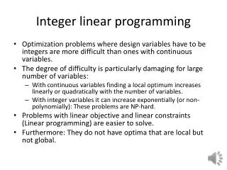
Introduction to Linear and Integer Programming
Introduction to Linear and Integer Programming. Saba Neyshabouri. Operations Research. OR was developed and used during world war II While the technology was advancing fast, the problems that analysts were facing were getting bigger and more complex.


Introduction to Linear and Integer Programming
E N D
Presentation Transcript
Introduction to Linear and Integer Programming Saba Neyshabouri
Operations Research • OR was developed and used during world war II • While the technology was advancing fast, the problems that analysts were facing were getting bigger and more complex. • Decision making for complex systems are very complicated and is out of human’s mind capability to solve problems with many variables. • Operations Research and optimization methods try to find “The Best” solution for a problem.
Operation Research • The founder of the field is George B. Dantzig who invented Simplex method for solving Linear Programming (LP) problems. • With Simplex it was shown that the optimal solution of LP’s can be found.
LP Structure • There are 3 main parts that forms an optimization problem: • Decision Variables: Variables that represent the decision that can be made. • Objective function: Each optimization problem is trying to optimize (maximize/minimize) some goal such as costs, profits, revenue. • Constraints: Set of real restricting parameters that are imposed in real life or by the structure of the problem. Example for constraints can be: • Limited budget for a project • Limited manpower or resources • Being limited to choose only one option out of many options (Assignment)
General Form of LP • The general form for LP is: • (1) is the objective function • (2),(3) are the set of constraints • X: vector of decision variables (n*1) • C: vector of objective function coefficients (n*1) • A: Technology matrix (m*n) • b: vector of resource availability (m*1)
LP example • Production planning:a producer of furniture has to make the decision about the production planning for 2 of its products: work desks and lunch tables. There are 2 resources available for production which these products are using: lumber and carpentry. 20 units of each resource is available. Here is the table containing the data for the problem:
LP example • First table shows the selling prices of each product, and second table show the amount of each resource that is used to produce one unit of product as well as resource availability. The question is how many of each product should be produced in order to maximize the revenue? • To model this problem as a linear programming formulation we should define our decision variables:
Example Formulation • Defining the decision variables of the problem, the formulation will be: • (1) is the total revenue generated by producing x1 desks and x2 tables. • (2) is the constraint for the total number of lumbers that exists. • (3) is the constraint for the total carpentry hours available. • (4) is the non-negativity constraints, saying that production can not be negative.
Feasible Region • Feasible region is defined by the set of constraints of the problem, which is all the possible points that satisfy the all the constraints. • In production planning problem, the feasible set defined by the constraints looks like this plot:
Feasible Region • The red line represents the line for (2) • The green line represents the line for (3) • The region with blue line represents entire feasible region of the problem.
Geometric Solution • To find the solution of LP problems, the line for objective function should be plotted and the point in feasible region which maximize (minimize) the function is the solution. • Dashed parallel lines are representing the objective function line for 2 different values.
Simplex and LP • Solution of LP problems are always at the extreme points of the feasible region:
Simplex and LP • Knowing the structure of LP problems and where the solutions are, there are finite number of extreme points that need to be checked in order to find the optimal solution. • However the number of extreme points are finite, but for a problem with n variables and m constraints the upper bound for the number of extreme points is (n>m) : • Simplex is an algorithm that systematically explores the extreme points of the feasible region and moves from an extreme point to its improving neighbor.
LP Solution (Production Planning) • For the production planning example the solutions are: • Since the number of desks and tables can not be fractional, we might be able to round the solution down to get our integer solution, with a revenue of 210. • Does rounding the solution yield the optimal solution to integer problem?
Optimization Software • There are various optimization tools developed based on Simplex and other optimization algorithms that are developed for LP problems. • The MPL code for our example is : TITLE Production_Planning INDEX Product=(Desk,LunchTable); Resource=(Lumber, Carpentry); DATA Price[Product] = (15 , 20); Availability[Resource] = (20 , 20); Usage [Product, Resource]= (1 , 2, 2 , 1); VARIABLES X[Product]; MODEL Max Revenue= SUM (Product: Price * X); SUBJECT TO ResourceLevel[Resource]: SUM (Product: Usage * X) <= Availability; END
Integer Optimization • Many of decisions and variables in real cases are inherently integers. • In our example the number of products to be manufactured can not be fractional and it has to be integer. • Many of the problems that are faced in real cases, have choosing an option in their structure, for example: • Which stock to invest in • Which route to choose to move in • Which arc of the graph to choose
Integer Variables • The only difference between LP problems and IP problems in structure is the definition of the decision variables. • How ever this change will fundamentally change the characteristics of the problem in hand. • LP problems have a convex set as their feasible region while IP problems have set of integer vectors as their feasible region (non-convex). • Dealing with non-convex optimization problems are much harder than convex optimization problems.
How to Solve IP Problems • LP relaxation: LP relaxation of and IP problem is when we allow the variables to take on fractional values (Like our example). • The idea to solve IP problems is to solve series of specific LP problems which will guide us towards an integer feasible solution. • This method is called Branch-and-Bound. • In this method, we branch on fractional values and make them to be the lower or upper integer value. • It is important to note that rounding the LP solution will not necessarily give the optimal or even feasible solution.
Example (Revisited) • Remember we got 210 as our objective function by rounding down the LP solutions. • If we solve the same problem as an IP the optimal solution will be:
Important Characteristics of IP Problems • IP problems generally are much more complicated than LP problems. • Many of IP classes are known as NP-hard problems, which takes very long processing time for computers to find the optimal solution (Years, for problems of real case size). • There has been extensive research in this area in order to find ways to be able to tackle these problems. • Cutting Planes • Branch-and-Cut • Column Generation techniques • Branch-and-Price • Meta Heuristics