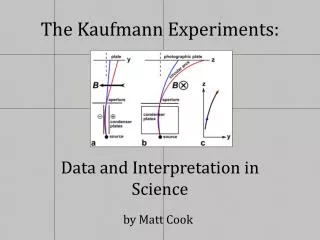
The Kaufmann Experiments
The Kaufmann Experiments. Cathy Huml Yao McCormick. The Kaufmann Experiments. Walter Kaufmann (1871-1947) Series of experiments aimed to determine the variation of an electron’s mass with its velocity.

The Kaufmann Experiments
E N D
Presentation Transcript
The Kaufmann Experiments Cathy Huml Yao McCormick
The Kaufmann Experiments • Walter Kaufmann (1871-1947) • Series of experiments aimed to determine the variation of an electron’s mass with its velocity. • Deals with Electron Theory of Matter, and the possible Electromagnetic origin for part or all of the mass of an electron.
Electromagnetic Mass of Electron • Competing Electromagnetic Mass Theories of the early 1900s. • The contenders: Walter Kaufmann (1871-1947), Max Abraham (1875-1922), Alfred Bucherer (1863-1927), Hendrik Lorentz (1853-1928), Max Planck (1858-1947).
Walter Kaufmann • Studied at the University of Berlin and Munich. • 1897-performed experiments on cathode rays and confirmed there existed negatively charged particles, but he didn’t believe that he was justified in calling them electrons.
Max Abraham • Studied at University of Berlin as Planck’s assistant. • In 1902 proposed his own model of the electron with charge uniformly distributed over the surface of a rigid sphere. • Opposed to Relativity, strong believer in the existence of the aether. • He loved his absolute aether, his field equations, his rigid electron just as a youth loves his first flame, whose memory no later experience can extinguish.
Alfred Bucherer • Studied at John’s Hopkins, Cornell, & Strasbourg. • Bucherer’s model of the electron was deformed as it moved through the aether, but in a fashion that its volume remained constant. • Kaufmann’s experiments could not distinguish between the models of Bucherer and Abraham.
Hendrik Lorentz • Lorentz model of the electron was based on a uniform spherical charge throughout the electron. • As an electron was set in motion through the ether its transverse dimensions remained unchanged but its length in the direction of motion contracted. • FitzGerald-Lorentz Contraction and the Special Theory of Relativity (Einstein-Lorentz Predictions)
Technical Details for Non-Physics People. (Like Myself) • Central Idea • Charge Q moving at a velocity of v which is small compared to the speed of light (c) • When v moves toward c, mass becomes very velocity dependent.
Kaufmann’s Experiments • Between 1901-1906, Kaufmann published a series of experiments that measured the variation of the charge to mass ratio of the electron. • From his experiments, Kaufmann discovered that the charge e of electron does not change with its velocity, v. • Decrease in the ratio e/m relates to the increase in m.
Kaufmann’s Experiments • Now e/m can be expressed in terms of coordinates ( y, z ). • y = (e/m)(A’/v2) = (e/m0)(A/c2)[1/(βψ(β))]z = (e/m)(A/v) = (e/m0)(A’/c)[1/(βψ(β))]With a function ψ(β) where m(v) = m0 ψ(β).
Kaufmann’s First Results • Kaufmann published his first results of e/m values for high-speed β rays ( 0.787 ≤ β ≤ 0.945 ) in his 1901 paper.
Kaufmann’s First Results • In his paper, Kaufmann tried to calculate the mechanical mass (“true” mass) and electromagnetic mass (“apparent” mass) of an electron.mtotal = Mtrue + mapparent • Kaufmann used Searle’s equation for total energy of a moving spherical electron to find mapparent = (1/v)(dW/dv), which is the longitudinal mass. • From his data points, Kaufmann calculated the “true” mass is about 3 times larger than the apparent mass.
Kaufmann’s 1902 Paper • Kaufmann’s 1901 analysis was incorrect because he used longitudinal mass rather than transverse mass. As well, his data points did not support relativity theory. • In 1902, Kaufmann published more data and analyzed in term of Abraham’s transverse mass. • Kaufmann corrected an algebraic error in his formula, and made some geometric change in the dimensions of his apparatus.
Kaufmann’s 1902 Paper • Because of rapid vibration in ψ(β), a small error in determining β would cause a huge uncertainty in m. Kaufmann declared that “The mass of the electrons that constitute the Becquerel rays is dependent on velocity. The dependency can be demonstrated exactly by the formula of Abraham. Therefore the mass of electron is purely of an electromagnetic nature.”
Kaufmann’s 1903 and 1905 Data • Kaufmann published more data in 1903 • In 1905, he published a set of 9 famous data points later Planck used to in his analysis
Kaufmann’s 1905 Paper • Kaufmann concluded his 1905 paper“The prevalent results decidedly speak against the correctness of Lorentz’s assumption as well as Einstein’s. If on account of that one considers this basic assumption refuted, then one would be forced to consider it a failure to attempt to base the entire field of physics, including electrodynamics and optics, upon the principle of relative movement. A choice between the theory of Abraham and Bucherer for the time being is impossible and does not seem to be attainable by observations of the type described above due to the largely numerical identity of the values of ψ(β). Whether Bucherer’s formula for the optics of movie bodies in the realm of possible observation can yield the same results as Lorentz’s, still has yet to be proven.”
Planck’s Analysis • Does Kaufmann’s data really give conclusive support of Abraham’s theory and equation for the variation of the electromagnetic mass of the electron? • Lorentz challenge and conclusion. • Planck’s challenge and conclusion.
Planck’s Analysis • Reversed interpretation of Kaufmann’s data. • “To be sure, this question [of the acceptability of the relativity principle] appears to be already answered through the recent and important measurements of W. Kaufmann, that is, however in the negative sense so that every further investigation seems to be unnecessary. In the meantime I would still like to consider it possible, in view of the extremely complex theory of these experiments, that the principle of relativity could be reconciled with these observations if one would more carefully elaborate them.”
Planck’s Analysis • How? • Planck computed the expected deflection on the basis of the Abraham and Lorentz theories.
Planck’s Analysis 1906 • Planck used Kaufmann’s 9 data points to compute a value u. • u=m0c/p
Planck’s Analysis • 1. Had value of e/m from Kaufmann. • 2. Obtain expression for p ( the radius of the spherical electron). • 3. Obtained values of B=v/c for each theory. • 4. Obtain values for y. • 5. Use his own equations for z and y to calculate B independently.
Planck’s Analysis • 3 MAIN ISSUES • 1. Uniform Electric Field • 2. Maintaining the Vacuum • 3. Kaufmann’s analysis Begs the Question
Planck’s Analysis • Reanalyze Kaufmann’s Data (1907) • Make Changes • Detect electric field at each distinct data point (y, z) • Found that Lorentz Theory more accurate detection of electric field, therefore favored by Kaufmann data. • Most Important: Kaufmann Experiments are no longer an obstacle in the path of the Theory of Relativity
Subsequent Determinations of e/m0 • It was still not clear whether Abraham’s or Lorentz’s theory was more correct, even after Plank’s reanalysis of Kaufmann’s data. • To prove the more favorable theory, other scientists Bestelmeyer, Bucherer, and Neumann did their own experiments.
Adolf Bestelmeyer • 1907, Adolf Bestelmeyer (1875-1954) used the secondary cathode rays ejected from a metal by incident X rays. • He measured the e/m for those electrons that were sent through the velocity selector (acted by crossed electric and magnetic fields), then deflected by magnetic field.
Adolf Bestelmeyer These data still did not show the clear favorite of these two theories, Abraham’s and Lorentz’s.
Alfred Bucherer • Like Bestelmeyer did, in 1909, Alfred Bucherer used β rays from a radium fluoride source through the velocity selector of crossed electic and magnetic fields.
Alfred Bucherer • Bucherer discovered that as β varies, the values for e/m0 stay nearly constant. • His data showed e/m0 is more constant for Lorentz’s theory than Abrahams, but there were still some controversies about his conclusion.
Neumann • 1914, Neumann finally found Lorentz’s theory has the most constant e/m0 values for different β. • Using am improved Bucherer’s method, he found 26 data points from 0.39152 ≤ β ≤ 0.80730, and did a best-fit graph of the points for both theories.
Neumann The best-fit graph favored Lorentz’s theory. It showed that Lorentz’s numbers were more accurate.
Mr. Einstein’s Thoughts… • On the Theories of Abraham and Bucherer… • On his Theory of Relativity…
In Conclusion • The Kaufmann experiments were a case study to illustrate the development and acceptance of scientific theory. • Experiment does not always yield a definitive result.