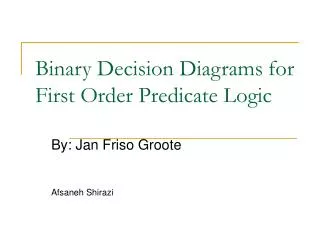
Binary Decision Diagrams for First Order Predicate Logic

1. Binary Decision Diagrams for First Order Predicate Logic By: Jan Friso Groote Afsaneh Shirazi

2. BDDs for FOL • First order predicate logic • Binary Decision Diagrams • Simple operations on BDDs • Advanced operations on BDDs • Algorithm • Example

3. First Order Predicate Logic • V : variables , F : functions , Pr : predicate symbols • Terms: • x  V is a term • If f  F is a function symbol of arity r and t1,…, tr are terms, then f(t1,…, tr)is a term • Set of all terms over F and V is denoted by T(F,V) • Set of all predicates of the form P(t1,…,tr) is denoted by P(Pr, F, V)

4. Substitution • Substitution is a mapping :V  T(F,V) • [x1:=t]: maps each variable x to (x), except x1 to t • Composition:  o (t) = ((t)) • We assume that  is extended : term to term, predicates to predicates

5. Formulas • Formulas are defined by: • t, f • P(t1, …, tr)  P(Pr, F, V) •  is a formula  is a formula •  and  are formulas     is a formula •  is a formula, and x  V is a variable  x. and x. are formulas • Set of all formulas: F (Pr, F, V)

6. Structure and Interpretation • A Structure is a ,multi-tuple  = <A; R1, R2,…;F1, F2,…> where • A is a non empty set • R1, R2,… are relations on A • F1, F2,… are functions on A • Herbrand structures have the form H= <T(F,); R1, R2,…;f1, f2,…> • Let  be a structure and  : V  A be a valuation. The interpretation : T(F, V)  A of a term t is defined: • if x V

7. Interpretation of a formula • F (Pr, F, V)  {0,1}

8. FOL • , ╞  iff • ╞  iff  , ╞  •  unsatisifiable iff for each  there is a valuation , , ╞ 

9. equivalency •    strongly (logically) equivalent  (,╞  iff ,╞ ) •    logically equivalent  (╞  iff ╞ ) •    weakly (logically) equivalent   ,╞  iff  ,╞  • No free variables: strong logical equivalence and logical equivalence coincide

10. Binary Decision Diagrams • A BDD, is an acyclic, node labeled graph where • Q : finite set of nodes • l : Q {0, 1}  P(Pr, F, V)  {0, 1} is a node labeling, that l(q)  0, 1 for all qQ • is the false continuation of a node • is the true continuation of a node • s  Q {0, 1} is a start node • 0 is a symbol representing false, and 1 representing truth • Each sequence q0 q1 … is bounded

11. Interpretation of a BDD • Let B be a BDD,  be astructure and  be a valuation. A , -path of a node q0  Q is the sequence where qn  {0,1} and for each i, i = f if ,  ╞ l(qi) and i = t if , ╞ l(qi) • If q0 ends in 1 we say that q0 holds, ,  ╞ q0 • So, A BDD yields a truth value.

12. BP(t1, …, tr) = 0 1 P(t1,…,tr) Bf = Bt = 0 1 then B = If B = 0 1 1 0 If B = and B = then B = 0 1 0 1 0 1 0 1

13. Example P(x) P(x) Q(y) P(x) R(z) 0 1 0 0 1

14. BDD • Let be a (quantifier free) formula and B its corresponding BDD. For each structure  and each valuation  we find that , ╞  iff , ╞ B • Proof: Straightforward on the structure of 

15. BDDs for FOL • First order predicate logic • Binary Decision Diagrams • Simple operations on BDDs • Advanced operations on BDDs • Algorithm • Example

16. Neglect Operator • Let be a BDD. Neglect operator is defined for some q,p q, p q by:

17. p,q-join Operator • If then

18. f-merge and f-sort operators • f-merge and f-sort operators, sort the BDD such that labels occur in ascending order. • Sorting a BDD is NP-hard • Avoid sorting a BDD

19. f-merge Operator • If then

20. f-sort Operator • If then

22. Simple Operations on BDDs • Lemma: (Soundness) Let B be a BDD. In case O is applicable to B, O(B)  B (O is one of ) Proof: check that for all structures and valuations  , ╞ O(B) iff  , ╞ B • Definition: B is reduced iff non of the operators is applicable

23. Simple Operations on BDDs • Lemma: Let B, C be BDDs pQB and qQC .Let  be a structure and  a valuation such that  , ╞ p and ,  ╞ q. P(t1,…,tn) : label not occurring in subdags p and q. Then • Exists a structure  and a valuation  , ╞ p, , ╞ q and , ╞ P(t1,…,tn) • Exists a structure  and a valuation  , ╞ p, , ╞ q and , ╞ P(t1,…,tn)

24. Simple Operations on BDDs • Lemma:Let B and C be reduced BDDs. pQB and qQC such that p  q. Then, • l(p) = l(q) • pf  qf • pt  qt • If B,C are the same, then p=q back

25. Isomorphism • Let B and C be BDDs. f: QB{0B,1B}  QC{0C,1C} is called homomorphism iff lC(f(p))=lB(p), f(pf ) = f(p)f and f(pt) = f(p)t . In case f is bijective, f is called isomorphism. • B = C (isomorphic) if there exists an isomorphism f.

26. Example C B f P(x) P(x) Q(x) Q(x) 0 1 0

27. Theorem • B and C are reduced BDDs, B  C. Then B = C (isomorphic). • Proof back

28. Theorem • Operators can be applied a finite number of times to B. • Proof back

29. R(B) • Let B be a BDD, C be a reduced BDD, B  C. According to theorem C is unique up to an isomorphism and It can be efficiently obtained (Thrm)  R(B) for C • R(B) = Bt ( tautology) • R(B) = Bf ( contradiction) • Basis for Propositional Logic

30. Advanced Operations on BDDs • Copying Operator C(B): puts B in conjunction with a copy of itself (different variables) • Unification Operator U(B): instantiate B according to  ( is a relevant unifier)

31. Copy Operator • Let B be a BDD in which variables occur. not occurring in B

32. Unifier • A substitution  is called a unifier of P(t1, …, tn) and Q(u1, …, um) iff (P(t1,…, tn))=(Q(u1,…,um)) • A unifier is most general (MGU) iff for each unifier ’ of P(t1,…, tn) and Q(u1,…,um) there is a substitution  such that  o  = ’ • Idempotent MGU:  ((x)) = x • Linear time

33. Relevant Unifier • A node p of B is redundant iff pt  pf • A path is allowed iff there are no i, j such that l(pi)=l(pj) and i  j • A node is truth-truth capable iff there is an allowed path

34. Relevant Unifier • A valuation  is a relevant unifier iff pi is not redundant, if i = f, pi is not truth-truth capable, and for some i, j, i = f, j = t and  is an idempotent MGU of l(pi) and l(pj).

35. Lemma • Let B be a reduced BDD. • No redundant nodes • Every path allowed • If pi is not truth-truth capable pit = 0 •  is a relevant unifier iff for some i, j, i=f, j=t and  is the MGU of l(pi) and l(pj) on the rightmost path of B

36. MGU y = a

37. Unification Operator • If  is a relevant unifier of B • Lemma: (Soundness) • B C(B) • B B U(B) • Proof: easy logical consequence back

38. BDDs for FOL • First order predicate logic • Binary Decision Diagrams • Simple operations on BDDs • Advanced operations on BDDs • Algorithm • Example

39. Algorithm Avoid expensive sorting operator All pairs of pi, pj in the rightmost path, with pit=0 and pjt0  Linearly in size of terms

40. Algorithm The depth of recursive calls is limited by the number of free variables Avoid sorting by grouping predicates with the same predicate symbol

41. Algorithm

42. Algorithm • The program is browsing through larger and larger BDDs of the form • We stop: • Bf Lemma • Bt

43. Russel’s Paradox • A set which contains those sets that are not members of themselves • F(x,y): x is a member of y • Problem: • negated and Skolemised formula

44. Russel’s Paradox (y) = a Example

45. Thank You Any Question?

46. Appendix A • Thrm: B and C are reduced BDDs, B  C. Then B = C (isomorphic). • Proof: Define f: QBQC and g: QCQB f(p) = q such that p  q g(q) = p such that p  q f is a homomorphism, g is the inverse of f  f is an isomorphism We assumed f and g are well defined.

47. Proof • B  C and all nodes in B are reachable from the root  each node in B is related via  to 1 node in C • p related to q1,q2  q1 q2 •  q1 = q2 (using thrm) back

48. Appendix B Proof: The transformation operators can be formulated as rewrite rules.l1 and l2 are predicates. l1 > l2

49. Proof • To each DAG we can obtain its canonical tree by undoing the sharing of subdags. Application of these rules must terminate on these trees. • Each rewrite of the DAG corresponds to one or more rewrite of canonical tree. • In Join operator the number of nodes are strictly decreasing  It should terminate back

50. Appendix C • A set is circular if it is a member of another set, which in turn is a member of the original. • There is no set containing all non circular sets. • Problem: • negated and Skolemised formula (a, f are skolem functions)