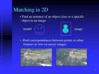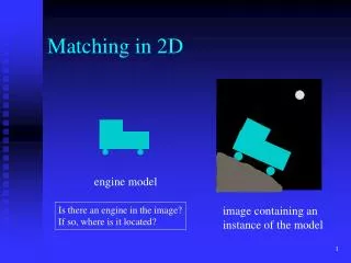
Matching in 2D
Matching in 2D. Mapping: Scaling Rotation Translation Warp. Introduction. How to make and use correspondences between images and maps, images and models, images and other images All work is done in two dimensions. Registration of 2D Data.

Matching in 2D
E N D
Presentation Transcript
Matching in 2D Mapping: Scaling Rotation Translation Warp
Introduction • How to make and use correspondences between • images and maps, • images and models, • images and other images • All work is done in two dimensions
Registration of 2D Data Equation and figure show an invertible mapping points of a model M and points of an image I. Actually, M and I can be any 2D coordinate space and each represent a map, amodel, or image. The mapping is invertible: functions g-1 and h-1 exist. Image registration is the process by which points of two images similar viewpoints of essentially the same scene are geometrically transformed so that corresponding feature points of the two images have the same coordinates after transformation.
Representation of points • A 2D point has two coordinates and is conveniently represented as either a row vector P=[x,y] or column vector P=[x,y]t . • Homogeneous Coordinates: It is often convenient notationally for computer processing to use homogeneous coordinates for points, especially when affine transformations are used. The homogeneous coordinates of a 2D point P=[x,y]t are [sx,sy,s]t, where s is a scale factor, commonly 1.0
AFFINE MAPPING FUNCTIONS • A large class of useful spatial transformations can be represented by multiplication of a matrix and a homogeneous point. • Scaling • Rotation • Translation
Scaling • A common operation is scaling • Uniform scaling changes all coordinates in the same way, or equivalently changes the size of all objects in the same way. • Figure shows a 2D point P=[1,2] scaled by a factor of 2 to obtain the new point P’=[2,4].
Scaling • Scaling is a linear transformation, meaning that it can be easily represented in terms of the scale factor applied to the two basis vectors for 2D Euclidean space. For example, [1,2]=1[1,0]+2[0,1] and 2[1,2]=2(1[1,0]+2[0,1] )=[2,4]
Rotation • A second common operation is rotation about a point in 2D space. • Figure shows a 2D point P=[x,y] rotated by angle θ counterclockwise about the origin to obtain the new point P’=[x’,y’].
Rotation • As for any linear transformation, we take the columns of the matrix to be the result of the transformation applied to the basis vectors; transformation of any other vectors can be expressed as a linear combination of the basis vectors.
Orthogonal and Orthonormal Transformations • Orthogonal A set of vectors is orthogonal if all pairs of vectors in the set are perpendicular (have scalar product of zero). • Orthonormal A set of vectors is orthonormal if it is an orthogonal set and all vectors have unit length. • A rotation preserves both the length of the basis vectors and their orthogonality.
Translation • Often, point coordinates need to be shifted by some constant amount, which is equivalent to changing the origin of the coordinate system. • Since translation does not map the origin [0,0] to itself, we cannot model it using a simple 2x2 matrix as has been done for scaling and rotation: In other words, it is not a linear operation.
Translation • The matrix multiplication shown in equation can be used to model the translation D of point[x,y] so that [x’,y’]=D([x,y])=[x+x0,y+y0]
Exercise: Rotation about a point • Give the 3x3 matrix that represents a π/2 rotation of the plane about the point [5,8] . • Hint: First derive the matrix D-5,-8 that translates the point [5,8] to the origin of a new coordinate frame. The matrix which we want will be the combination D5,8Rπ/2D-5,-8 • Check that your matrix correctly transforms points [5,8], [6,8] and [5,9].
Rotation,Scaling and Translation • Figure shows a common situation: An image I[r,c] is taken by a square-pixel camera looking perpendicularly down on a planar workspace W[x,y]. This conversion can be done by composing a rotation R, a scaling S and a translation D as given and denoted wPj=Dx0,y0SsRθiPj.
Rotation,Scaling and Translation • For example, we have • iP1=[100,60] and wP1=[200,100]. • iP2=[380,120] and wP2=[300,200]. • Control points are clearly distinguishable and easily measured points to establish known correspondences between different coordinate spaces. • θ is easily determined independent of the other parameters as follows: • θi=arctan((iy2-iy1)/(ix2-ix1)) θi=arctan(60/280)=12.09o • θw=arctan((wy2-wy1)/(wx2-wx1)) θw=arctan(100/100)=45o • θ= θw- θi θ=32.91o • Once θ is determined, all sin andcos elements are known: There are 3 equations and 3 unknowns which can be solved for s and x0 ,y0.
Object Recognition and Location Example (left) Model object and (right) three holes detected in an image
Object Recognition and Location Example We will use the hypothesized correspondences (A,H2) and (B,H3) to deduce the transformation
Object Recognition and Location Example • The direction of the vector from A to B in the model is θ1=arctan(9.0/8.0)=0.844 • Corresponding vector from H2 to H3 in the image θ2=arctan(12.0/0.0)= π/2=1.571 • The rotation is thus θ=0.727 radians • The known matching coordinates for points A in the model and H2 in the image, we obtain the following system, where u0,v0 are the unknown translation components in the image plane. The two resulting equations readily produce u0=15.3 and v0=-5.95
Object Recognition and Location Example • Having a complete spatial transformation, we can now compute the location of any model points in the image space, including the grip points R=[29,19] and Q=[32,12]. • As shown next, model point R transforms to image point iR=[24.4, 27.4] • Using Q=[32,12] as the input to the transformation outputs the image location iQ=[31.2, 24.2] for the other grip point.
2D OBJECT RECOGNITION VIA AFFINE MAPING • Methods of recognizing 2D objects through mapping of model points onto image points • Local-Feature-Focus Method • Pose-Clustering Algorithm • Geometric Hashing The methods are meant to determine if a given image contains an instance of an object modeland to determine the pose(position and orientation) of the object with respect to camera.
2D OBJECT RECOGNITION VIA AFFINE MAPING A 2D model and 3 matching image of an airplane part
Pose Clustering • We have seen that an alignment between model and image features using an RST transformation can be obtained from two matching control points. • Obtaining the matching control points automatically may not be easy due to ambiguous matching possibilities. • The pose-clustering approach computes an RST alignment for all possible control point pairs and then checks for a cluster of similar parameter sets.
Example Pose Detection Problem Assume that the pairs of combined type LX or TY are used in this example