Download
1 / 54
590 likes | 1.07k Vues
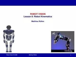
ROBOT VISION Lesson 8: Robot Kinematics Matthias Rüther. Contents. Introduction Overview Basic Terms Typical Configurations Geometry Homogeneous Transformations Representing Orientation Direct Kinematics Open Chain Denavit-Hartenberg Typical Configurations Inverse Kinematics Problem

E N D
Contents • Introduction • Overview • Basic Terms • Typical Configurations • Geometry • Homogeneous Transformations • Representing Orientation • Direct Kinematics • Open Chain • Denavit-Hartenberg • Typical Configurations • Inverse Kinematics • Problem • Numerical Algorithms
Overview • An industrial robot consists of • A manipulator that consists of a sequence of rigid bodies (links) connected by means of articulation (joints). It is characterized by an arm (for mobility), a wrist (for dexterity) and an end effector (to perform a task). • Actuators that set the manipulator in motion by actuating the joints (electric, hydraulic or pneumatic) • Sensors that measure the manipulators status (proprioceptive sensors) or the status of the environment (exteroceptive sensors). • A control system that controls and supervises manipulator motion.
Overview • An industrial robot has three fundamental capacities • Material handling: objects are transported from one location to another, their physical characteristics are not altered (e.g. pallettizing, warehouse loading/unloading, sorting, packaging) • Material Manipulation: physical characteristics of objects are changed or their physical identity is lost (e.g. welding, painting, gluing, cutting, drilling, screwing, assembly, …) • Measurement: object properties are measured by sensors on the end effector, so they are able to explore a 3D environment (e.g. quality control by image processing, tactile sensors, …)
Basic Terms • Kinematic chain: sequence of links and joints connecting the end effector to the base. Can be open (single chain) or closed (loop within the chain). • Joints: • Revolute: rotational joint • Prismatic: translational joint • Degree of mobility: each joint typ. provides an additional DOM (e.g. 6DOM necessary for 3D motion) • Accuracy: „How close does the robot get to a desired point?“, distance between desired point and actual point. (off line) • Repeatability: „How close does the robot get to a position it has reached before?“ (on line)
Repeatability and Accuracy Repeatability: the measurement of how closely a robot returns to the same positionn number of times. Accuracy: the measurement of how closely the robot moves to a given target coordinate. Where: Ptis the target position, Pathe average achieved position, R is the repeatability, and A is the accuracy.
Many factors can effect the accuracy of a robot such as: • environmental factors (eg temperature, humidity and electrical noise); • kinematic parameters (eg robot link lengths etc); • dynamic parameters (eg structural compliance, friction); • measurement factors (eg resolution and non-linearity of encoders and resolvers); • computational factors (eg digital round off, steady-state control errors); and • application factors (eg installation errors and errors in defining work-piece coordinate frames).
Why? Each of these can effect the robot kinematics • depending on the robot model design and manufacturing process the kinematics can be the most significant source of error. • if the internal kinematic model of the robot does not match the actual model we can not accurately predict where the end-effector is. Make them match by either • tighter manufacturing tolerances; or • by measuring actual kinematics and incorporating this information into the kinematic model.
Basic Terms • Joint space: end effector position and orientation given in joint coordinates. • Operational space: end effector position and orientation given in world coordinates (e.g. cartesian coordinate system) • Workspace: • Reachable WS: set of positions the EE can reach • Dexterous WS: set of positions the EE can reach with a given orientation • Redundancy: more DOM than needed are available
Basic Joints Revolute Joint 1 DOF ( Variable - ) Prismatic Joint 1 DOF (linear) (Variables - d)
An Example - The PUMA 560 2 3 4 1 There are two more joints on the end effector (the gripper) The PUMA 560 hasSIXrevolute joints A revolute joint has ONE degree of freedom ( 1 DOF) that is defined by its angle
Joint 2 Joint 2 q2 Joint 3 Joint 3 q1 Joint 1 Joint 1 yt Tool Coordinate Frame Tool Coordinate Frame zt Link 1 Link 1 z1 z1 zw World (Base) Coordinate Frame World (Base) Coordinate Frame xw Forward and Inverse Kinematics Link Space n variables (q1 … qn) Tool Space 6 variables (x,y,z,qx,qy,qz) Forward K Inverse K
z y x z2 yt zt x2 Link frame Tool Coordinate Frame zw World (Base) Coordinate Frame xw Co-ordinate Frames • right handed coordinate frames • used as reference frames
F o r w a r d K i n e m a t i c s F o r w a r d K i n e m a t i c s
The Situation: You have a robotic arm that starts out aligned with the xo-axis. You tell the first link to move by 1 and the second link to move by 2. The Quest: What is the position of the end of the robotic arm? Solution: 1. Geometric Approach This might be the easiest solution for the simple situation. However, notice that the angles are measured relative to the direction of the previous link. (The first link is the exception. The angle is measured relative to it’s initial position.) For robots with more links and whose arm extends into 3 dimensions the geometry gets much more tedious. 2. Algebraic Approach Involves coordinate transformations.
Example Problem: You are have a three link arm that starts out aligned in the x-axis. Each link has lengths l1, l2, l3, respectively. You tell the first one to move by 1, and so on as the diagram suggests. Find the Homogeneous matrix to get the position of the yellow dot in the X0Y0 frame. Y3 3 2 3 X3 Y2 2 X2 H = Rz(1) * Tx1(l1) * Rz(2) * Tx2(l2) * Rz(3) i.e. Rotating by 1 will put you in the X1Y1 frame. Translate in the along the X1 axis by l1. Rotating by 2 will put you in the X2Y2 frame. and so on until you are in the X3Y3 frame. The position of the yellow dot relative to the X3Y3 frame is (l1, 0). Multiplying H by that position vector will give you the coordinates of the yellow point relative the the X0Y0 frame. Y0 1 X1 1 Y1 X0
Slight variation on the last solution: Make the yellow dot the origin of a new coordinate X4Y4 frame Y3 Y4 3 2 3 X3 Y2 2 X2 X4 H = Rz(1) * Tx1(l1) * Rz(2) * Tx2(l2) * Rz(3) * Tx3(l3) This takes you from the X0Y0 frame to the X4Y4 frame. The position of the yellow dot relative to the X4Y4 frame is (0,0). Y0 1 X1 1 Y1 X0 Notice that multiplying by the (0,0,0,1) vector will equal the last column of the H matrix.
More on Forward Kinematics… Denavit - Hartenberg Parameters
Denavit-Hartenberg Notation Z(i - 1) Y(i -1) Y i Z i X i a i a(i - 1 ) d i X(i -1) i ( i - 1) IDEA: Each joint is assigned a coordinate frame. Using the Denavit-Hartenberg notation, you need 4 parameters to describe how a frame (i) relates to a previous frame ( i -1 ). THE PARAMETERS/VARIABLES: , a , d,
The Parameters You can align the two axis just using the 4 parameters Z(i - 1) Y(i -1) Y i Z i X i a i a(i - 1 ) di X(i -1) i ( i - 1) 1) a(i-1) Technical Definition: a(i-1) is the length of theperpendicular between the joint axes. The joint axes is the axes around which revolution takes place which are the Z(i-1) and Z(i) axes. These two axes can be viewed as lines in space. The common perpendicular is the shortest line between the two axis-lines and is perpendicular to both axis-lines.
Z(i - 1) Y(i -1) Y i Z i X i a i a(i - 1 ) di X(i -1) i ( i - 1) a(i-1) cont... Visual Approach - “A way to visualize the link parameter a(i-1) is to imagine an expanding cylinder whose axis is the Z(i-1) axis - when the cylinder just touches the joint axis i the radius of the cylinder is equal to a(i-1).” (Manipulator Kinematics) It’s Usually on the Diagram Approach - If the diagram already specifies the various coordinate frames, then the common perpendicular is usually the X(i-1) axis. So a(i-1) is just the displacement along the X(i-1) to move from the (i-1) frame to the i frame.
Z(i - 1) Y(i -1) Y i Z i X i a i a(i - 1 ) di X(i -1) i ( i - 1) 2) (i-1) Technical Definition: Amount of rotation around the common perpendicular so that the joint axes are parallel. i.e. How much you have to rotate around the X(i-1) axis so that the Z(i-1) is pointing in the same direction as the Zi axis. Positive rotation follows the right hand rule. 3) d(i-1) Technical Definition: The displacement along the Zi axis needed to align the a(i-1) common perpendicular to the aicommon perpendicular. In other words, displacement along the Zi to align the X(i-1) and Xi axes. If the link is prismatic, then d(i-1) is a variable, not a parameter 4) i or i Amount of rotation around the Zi axis needed to align theX(i-1) axis with the Xi axis.
The Denavit-Hartenberg Matrix Just like the Homogeneous Matrix, the Denavit-Hartenberg Matrix is a transformation matrix from one coordinate frame to the next. Using a series of D-H Matrix multiplications and the D-H Parameter table, the final result is a transformation matrix from some frame to your initial frame. Z(i - 1) Y(i -1) Y i Z i X i a i a(i - 1 ) di X(i -1) i ( i - 1)
Y2 Z2 Z1 Z0 X2 d2 X0 X1 Y0 Y1 a1 a0 3 Revolute Joints Denavit-Hartenberg Link Parameter Table Notice that the table has two uses: 1) To describe the robot with its variables and parameters. 2) To describe some state of the robot by having a numerical values for the variables.
Y2 Z2 Z1 Z0 X2 d2 X0 X1 Y0 Y1 a0 a1 Note: T is the D-H matrix with (i-1) = 0 and i = 1.
This is just a rotation around the Z0 axis This is a translation by a0 followed by a rotation around the Z1 axis This is a translation by a1 and then d2 followed by a rotation around the X2 and Z2 axis
Review of Direct Kinematics • What we have: • Geometric layout of robot (constant under robot motion) • Joint positions qnx1 (variable under robot motion) • What we want: • End Effector (EE) position and orientation wrt base coordinate frame (variable under robot motion) • A coordinate transformation T from EE coordinates to base coordinates, where T is a function of q: • E.g. position of EE coordinate origin is:
Review of Direct Kinematics • How we get there: • Place local coordinate frame at each joint i, i=1..n: • Determine common normal (CN) between joint i and i-1 (i.e. line connecting both joint axes in the shortest possible way) • Place coordinate origin oi-1 at intersection of CN and joint axis i-1 • Attention Sciavicco/Siciliano: oi-1 at intersection of CN and joint axis i! • Set z-axis in direction of joint axis • Set x-axis in direction of CN • Model robot arm using Denavit-Hartenberg (DH) parameters: • a: shortest distance between consecutive joint axes (length of common normal CN). • : angle between consecutive joint axes around CN. • d: distance between consecutive coordinate origins along i-th joint axis (distance between i-th coordinate origin and intersection of CN with i-th joint axis. • y or : angle between consecutive CN‘s around joint axis. • Depending on joint type, either d or y are variables.
Review of Direct Kinematics • From DH-table, calculate T recursively:
Inverse Kinematics From Position to Angles K-1 (q1 … qn) (x,y,z,qx,qy,qz)
Inverse Kinematics • What we have: • Geometric layout of robot (constant under robot motion) • End Effector (EE) position and orientation wrt base coordinate frame (variable under robot motion) • What we want: • Joint coordinates qnx1 (variable under robot motion). • A mapping f from EE position and orientation to joint coordinates: • Problematic, because: • EE position may be out of reachable workspace (no solution) • EE position and orientation may be out of dexterous workspace (no solution) • EE position may be reachable in several ways (multiple solutions, redundancy) • EE position may be reachable in infinitely many ways (infinite number of solutions, redundancy) • f is highly nonlinear, no closed form solution for complicated configurations.
Inverse Kinematics • How we get there: • Calculate closed-form solution, if possible • fast • accurate • unique for every arm configuration (no general concept) • Use Iterative Method based on differential kinematics • slower • gives approximate solution • converges to a single solution (even if multiple solutions exist) • general algorithm, applicable to all arm configurations
Multiple Solutions • ·Because we are dealing with transcendental functions there is often more than one solution. • eg: cos-1(0.5) = 60º and 300º
A Simple Example Finding : Revolute and Prismatic Joints Combined More Specifically: (x , y) arctan2() specifies that it’s in the first quadrant Y Finding S: S 1 X
l2 l1 Inverse Kinematics of a Two Link Manipulator Given:l1, l2 ,x , y Find:1, 2 Redundancy: A unique solution to this problem does not exist. Sometimes no solution is possible. (x , y) 2 l2 l1 1 (x , y) l2 l1
The Geometric Solution l2 Using the Law of Cosines: 2 (x , y) l1 1 Using the Law of Cosines: Redundant since 2 could be in the first or fourth quadrant. Redundancy caused since 2 has two possible values
The Algebraic Solution (x , y) l2 2 l1 1 Only Unknown
We know what 2 is from the previous slide. We need to solve for 1 . Now we have two equations and two unknowns (sin 1 and cos 1 ) Substituting for c1 and simplifying many times Notice this is the law of cosines and can be replaced by x2+ y2
A General Solution • A general solution to the IK problem is obtained using differential kinematics. • There exists a linear mapping between EE velocity and Joint velocity. • Joint positions can be computed by integrating velocities over time.
Differential Kinematics • What we have: • Geometric layout of robot (constant under robot motion) • Joint velocities • What we want: • Linear velocity • Angular velocity • A mapping J from joint velocities to EE velocities:
The Jacobian • Jacobian matrix J(q) gives linear and angular velocity (p‘, ) as a function of joint velocity (q‘) • Depends on the location in joint space, hence J(q) • Can be computed via closed formula.
Derivative of a Rotation Matrix • Consider rotation matrix R(t), what is its derivative? • Interpretation of S: S is the cross-matrix of angular velocities
Example: rotation about z-axis • We want to compute the time-derivative of Rz(t)
Velocity composition rule • Consider the coordinate transformation of a point P from coordinate frame 1 to frame 0: origin of 1 wrt 0 rotation of 1 wrt 0 point wrt 1 point wrt 0 If p1 is fixed:
Link Velocity • Consider link i connecting joints i and i+1 with their coordinate frames • Let pi and pi+1 be the coordinate frame origins wrt base coordinate frame • Let rii,i+1 be the coordinate frame origin of i+1 wrt coordinate frame i, expressed in coordinate frame i Lin. velocity of i Lin. velocity of i+1 wrt i Angular velocity of i Lin. velocity of i+1 … angular velocity (without derivation) Angular velocity of i+1 Angular velocity of i Angular velocity of i+1 wrt i
Link Velocity • For prismatic joint: • For revolute joint:
Computation of Jacobian • Let the Jacobian J be partitioned into the following 3x1 vectors: • Prismatic joint: • Revolute joint: … contribution of joint i to EE linear velocity … contribution of joint i to EE angular velocity