Parallel and Distributed Simulation

1. Parallel and Distributed Simulation Time Parallel Simulation

2. Outline • Space-Time Framework • Time Parallel Simulation • Parallel Cache Simulation • Simulation Using Parallel Prefix

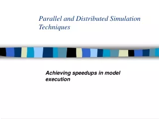
3. space-parallel simulation (e.g., Time Warp) LP1 LP2 region in space-time diagram LP3 physical processes physical processes LP4 LP5 inputs to region LP6 simulated time simulated time Space-Time Framework A simulation computation can be viewed as computing the state of the physical processes in the system being modeled over simulated time. algorithm: 1. partition space-time region into non-overlapping regions 2. assign each region to a logical process 3. each LP computes state of physical system for its region, using inputs from other regions and producing new outputs to those regions 4. repeat step 3 until a fixed point is reached

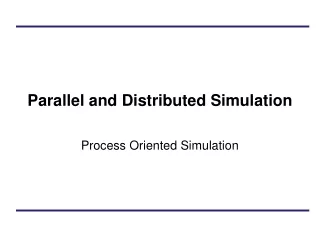
4. processor 1 processor 2 processor 3 processor 4 processor 5 possible system states simulated time Time Parallel Simulation Observation: The simulation computation is a sample path through the set of possible states across simulated time. Basic idea: • divide simulated time axis into non-overlapping intervals • each processor computes sample path of interval assigned to it Key question: What is the initial state of each interval (processor)?

5. processor 1 processor 2 processor 3 processor 4 processor 5 possible system states simulated time Time Parallel Simulation: Relaxation Approach 1. guess initial state of each interval (processor) 2. each processor computes sample path of its interval 3. using final state of previous interval as initial state, “fix up” sample path 4. repeat step 3 until a fixed point is reached Benefit: massively parallel execution Liabilities: cost of “fix up” computation, convergence may be slow (worst case, N iterations for N processors), state may be complex

6. Example: Cache Memory • Cache holds subset of entire memory • Memory organized as blocks • Hit: referenced block in cache • Miss: referenced block not in cache • Replacement policy determines which block to delete when requested data not in cache (miss) • LRU: delete least recently used block from cache • Implementation: Least Recently Used (LRU) stack • Stack contains address of memory (block number) • For each memory reference in input (memory ref trace) • if referenced address in stack (hit), move to top of stack • if not in stack (miss), place address on top of stack, deleting address at bottom

7. first iteration: assume stack is initially empty: 1 - - - 2 1 - - 1 2 - - 3 1 2 - 4 3 1 2 3 4 1 2 6 3 4 1 7 6 3 4 2 - - - 1 2 - - 2 1 - - 6 2 1 - 9 6 2 1 3 9 6 2 3 9 6 2 6 3 9 2 4 - - - 2 4 - - 3 2 4 - 1 3 2 4 7 1 3 2 2 7 1 3 7 2 1 3 4 7 2 1 address: 1 2 1 3 4 3 6 7 2 1 2 6 9 3 3 6 4 2 3 1 7 2 7 4 9 6 2 1 1 3 2 4 LRU Stack: processor 1 processor 2 processor 3 second iteration: processor i uses final state of processor i-1 as initial state address: 2 7 6 3 1 2 7 6 2 1 7 6 6 2 1 7 9 6 2 1 4 6 3 9 2 4 6 3 3 2 4 6 1 3 2 4 1 2 1 3 4 3 6 7 2 1 2 6 9 3 3 6 4 2 3 1 7 2 7 4 (idle) LRU Stack: match! match! processor 1 processor 2 processor 3 Given a sequence of references to blocks in memory, determine number of hits and misses using LRU replacement Example: Trace Drive Cache Simulation Done!

8. Outline • Space-Time Framework • Time Parallel Simulation • Parallel Cache Simulation • Simulation Using Parallel Prefix

9. + + + + + + + + + + + + + X1 X2 X3 X4 X5 X6 X7 X8 add value one position to the left + + + + 1,2 2,3 3,4 4,5 5,6 6,7 7,8 add value two positions to the left 1-3 1-4 2-5 3-6 4-7 5-8 add value four positions to the left 1-3 1-4 1-5 1-6 1-7 1-8 1 1-2 Time Parallel Simulation Using Parallel Prefix Basic idea: formulate the simulation computation as a linear recurrence, and solve using a parallel prefix computation parallel prefix: Give N values, compute the N initial products P1= X1 P2= X1 • X2 Pi = X1 • X2 • X3 • … • Xi for i = 1,… N; • is associative Parallel prefix requires O(log N) time

10. Example: G/G/1 Queue Example: G/G/1 queue, given • ri = interarrival time of the ith job • si = service time of the ith job Compute • Ai = arrival time of the ith job • Di = departure time of the ith job, for i=1, 2, 3, … N Solution: rewrite equations as parallel prefix computations: • Ai = Ai-1 + ri (= r1 + r2 + r3 + … ri) • Di = max (Di-1 , Ai ) + si

11. Summary of Time Parallel Algorithms • Pro: • allows for massive parallelism • often, little or no synchronization is required after spawning the parallel computations • substantial speedups obtained for certain problems: queueing networks, caches, ATM multiplexers • Con: • only applicable to a very limited set of problems