Download
1 / 41
410 likes | 513 Vues
Investigating wind-driven circulation and headland eddies' role in larval dispersal along irregular coastlines using idealized ROMS simulations. Study aims to determine connectivity patterns under various wind regimes.

E N D
Quantitative Description of Particle Dispersal over Irregular Coastlines Tim Chaffey, Satoshi Mitarai, Dave Siegel
BACKGROUND • Topographic eddies may be important in determining habitat connectivity • Eddies can retain larvae for time scales comparable with their PLD • High local recruitment is observed in island wake eddies (e.g., Swearer et al, 1999) • But, such clear pattern will not be observed in coastal eddies where currents are less persistent in direction (Graham & Largier, 1997) • Filament formation may be important in offshore transport of larvae (Haidvogel, 1991) • Offshore filaments present an obstacle to nearshore settlement in PLD. • Few notable studies (Largier, 2003) • Geostrophic size & flow time scale considered
GOAL OF THIS STUDY • Use coastal 3-D physical model to investigate the wind driven circulation around idealized irregularities in the coastline. • Estimate the role of coastal headland eddies on larval dispersal usingidealized ROMS simulations • Do headlands create a consistent connectivity or a stochastic connectivity? • Are the spatial scales of settlement similar to the straight coastline case (50 km)? • If there is a consistent connectivity, does it remain constant under different wind regimes? • Is there a critical headland amplitude/width? • How important is headland spacing? • Describe the physics of filament formation and eddy recirculation around headlands? • Can we develop theoretical relationships between headland size, wind forcing, bathymetry and release-settlement relationship? • If we can develop theory, we can use this theory to predict release-settlement relationships over realistic coastlines given wind, headland size, and bathymetry.
How this all comes together 1 - Collect CalCOFI data (SSH, temperature), bathymetry data, wind data from buoys. 2 - Initialized three-dimensional coastal circulation model (ROMS) with above data. 3 - Use 3D flow, 3D temperature, and SSH from model to compute flow statistics offline (Matlab). 4 - Use 3D flow from model to track particles offline (Matlab). We have ultimate flexibility in how we manipulate particles.
Model Setup • Wind field from buoy measurements • Wind field sum of a mean and perturbation component • July wind field (upwelling period) • Pressure gradient quantified using dynamic height data from CalCOFI July ship track survey. • Pressure gradient rotated to along the coast line inside the 500 m isobath Domain: 288 km Cross-shore, 256 km Alongshore • Bathymetry - 0 m to 500 m offshore • Irregular coastline (headland) created using a Gaussian function
HEADLAND DESIGN • Gaussian-shape headland in idealized simulations • Three parameters 3. Domain size (d) = distance between headlands 1. Amplitude (a) 2. Width (w) (twice the std of Gaussian function) a = 20 km w = 20 km d = 256 km
Variable Model Parameters • Wind Field • Uniform - Wind field principal axis has uniform (N-S) direction over domain • Alongshore - Wind field principal axis rotated to follow land inside 500 m isobath • Pressure Gradient • Alongshore - Pressure gradient principal axis rotated to follow land inside 500 m isobath • Bathymetry • Compression - Distance from land to 500 m isobath compresses near headland • Alongshore- Distance from land to 500 m isobath same at all points.
Wind Alongshore Uniform Compression BC - WA BC - WU Bathymetry Alongshore BA - WA BA - WU Notation for Cases Tested
Particle Tracking • 90,000 particles randomly released 10 km from land and in the upper 10 m, but with a uniform release distribution over 90 days. • Particles locations updated every three hours. • Particles settle when within competency window and 10 km of land. • Particles are treated as packets that can settle multiple times. • Particle bouncing schemes vary • Reflecting - particles are reflected off boundary • Non-reflecting - particles entering land are returned to prior time step over water
Wind Alongshore Uniform Compression BC - WA BC - WU Bathymetry Alongshore BA - WA BA - WU Model Parameters
BA-WA(1) BA-WA(2) BA-WA(3) Mean Connectivity, Reflecting Condition (∆t = 3 hr)
BA-WA(1) BA-WA(2) BA-WA(3) Arrival Diagram - Reflecting Condition
BA-WA(1) BA-WA(2) BA-WA(3) Mean Settler Dispersal Kernel - Reflecting Condition
BA-WA(1) BA-WA(2) BA-WA(3) Mean Connectivity, Non - Reflecting Condition (∆t = 3 hr)
BA-WA(1) BA-WA(2) BA-WA(3) Arrival Diagram - Non -Reflecting Condition
BA-WA(1) BA-WA(2) BA-WA(3) Mean Settler Dispersal Kernel - Non - Reflecting Condition
Wind Alongshore Uniform Compression BC - WA BC - WU Bathymetry Alongshore BA - WA BA - WU Model Parameters
BC - WU(1) BC - WU (2) Connectivity, Reflecting Condition (∆t = 3 hr)
BC-WU (1) BC-WU (2) Arrival Diagram - Reflecting Condition
BC - WU(1) BC - WU (2) Settler Dispersal Kernel - Reflecting Condition
BC - WU(1) BC - WU (2) Connectivity, Non-Reflecting Condition (∆t = 3 hr)
BC-WU (1) BC-WU (2) Arrival Diagram - Non -Reflecting Condition
Settler Dispersal Kernel - Non-Reflecting Condition BC - WU(1) BC - WU (2)
Summary • Dispersal for the alongshore wind cases are realistic while uniform wind cases are artificial. • For uniform wind cases, nearshore irregularities in the flow create artificial particle accumulation on the wayward side of the headland • A semi-annual pattern of dispersal is present in the alongshore wind case for both bathymetrys and both bouncing schemes. • For alongshore wind cases, particle dispersal over 1.5 years has a uniform distribution.
Future Work • Experiment with alternative bouncing scheme to remove artificial accumulation of particles • Compare time integrated temperature fields to CALCOFI data to validate simulations • Investigate vertical velocity at fixed depth and mixed layer depth to theoretical predications to validate simulations • Collaborate with Bernardo Broitman (NCEAS) to assess the variation of isobathic distances with coastline • Bridge the connections between headland size, flow structure, and dispersal. Time scales will be important!
Wind Alongshore Uniform Compression BC - WA BC - WU Bathymetry Alongshore BA - WA BA - WU Model Parameters
BC-WA(1) BC-WA(2) BC-WA(3) Mean Connectivity, Reflecting Condition (∆t = 3 hr)
BC-WA(1) BC-WA(2) BC-WA(3) Arrival Diagram - Reflecting Condition
BC-WA(1) BC-WA(2) BC-WA(3) Mean Settler Dispersal Kernel - Reflecting Condition
BC-WA(1) BC-WA(2) BC-WA(3) Mean Connectivity, Non-Reflecting Condition (∆t = 3 hr)
BC-WA(1) BC-WA(2) BC-WA(3) Arrival Diagram - Non - Reflecting Condition
BC-WA(1) BC-WA(2) BC-WA(3) Mean Settler Dispersal Kernel - Non - Reflecting Condition
Mean Dispersal Statistics • Mean alongshore distance - 35.9 km • Standard deviation of alongshore - 56.1 km • 11.5 % particles settle at least once • Mean PLD of settling particles 25.2 days (competency window = 20 - 40 days)