Download
1 / 34
370 likes | 673 Vues
Chapter 4 Introduction to Probability. Experiments, Counting Rules, and Assigning Probabilities. Events and Their Probability. Some Basic Relationships of Probability. Conditional Probability. Probability as a Numerical Measure of the Likelihood of Occurrence.

E N D
Chapter 4 Introduction to Probability • Experiments, Counting Rules, and Assigning Probabilities • Events and Their Probability • Some Basic Relationships of Probability • Conditional Probability
Probability as a Numerical Measureof the Likelihood of Occurrence Increasing Likelihood of Occurrence 0 .5 1 Probability: The event is very unlikely to occur. The occurrence of the event is just as likely as it is unlikely. The event is almost certain to occur.
An Experiment and Its Sample Space An experimentis any process that generates well-defined outcomes. The sample space for an experiment is the set of all experimental outcomes. An experimental outcome is also called a sample point.
Example: Bradley Investments Bradley has invested in two stocks, Markley Oil and Collins Mining. Bradley has determined that the possible outcomes of these investments three months from now are as follows. Investment Gain or Loss in 3 Months (in $000) Collins Mining Markley Oil 8 -2 10 5 0 -20
A Counting Rule for Multiple-Step Experiments • If an experiment consists of a sequence of k steps • in which there are n1 possible results for the first step, • n2 possible results for the second step, and so on, • then the total number of experimental outcomes is • given by (n1)(n2) . . . (nk). • A helpful graphical representation of a multiple-step experiment is a tree diagram.
A Counting Rule for Multiple-Step Experiments Bradley Investments can be viewed as a two-step experiment. It involves two stocks, each with a set of experimental outcomes. Markley Oil: n1 = 4 Collins Mining: n2 = 2 Total Number of Experimental Outcomes: n1n2 = (4)(2) = 8
Tree Diagram Collins Mining (Stage 2) Markley Oil (Stage 1) Experimental Outcomes Gain 8 (10, 8) Gain $18,000 (10, -2) Gain $8,000 Lose 2 Gain 10 (5, 8) Gain $13,000 Gain 8 (5, -2) Gain $3,000 Lose 2 Gain 5 Gain 8 (0, 8) Gain $8,000 Even (0, -2) Lose $2,000 Lose 2 Lose 20 Gain 8 (-20, 8) Lose $12,000 (-20, -2) Lose $22,000 Lose 2
Counting Rule for Combinations A second useful counting rule enables us to count the number of experimental outcomes when n objects are to be selected from a set of N objects. Number of Combinations of N Objects Taken n at a Time where: N! = N(N- 1)(N- 2) . . . (2)(1) n! = n(n- 1)(n- 2) . . . (2)(1) 0! = 1
Counting Rule for Permutations A third useful counting rule enables us to count the number of experimental outcomes when n objects are to be selected from a set of N objects, where the order of selection is important. Number of Permutations of N Objects Taken n at a Time where: N! = N(N- 1)(N- 2) . . . (2)(1) n! = n(n- 1)(n- 2) . . . (2)(1) 0! = 1
Assigning Probabilities Classical Method Assigning probabilities based on the assumption of equally likely outcomes Relative Frequency Method Assigning probabilities based on experimentation or historical data Subjective Method Assigning probabilities based on judgment
Classical Method If an experiment has n possible outcomes, this method would assign a probability of 1/n to each outcome. Example Experiment: Rolling a die Sample Space: S = {1, 2, 3, 4, 5, 6} Probabilities: Each sample point has a 1/6 chance of occurring
Relative Frequency Method • Example: Lucas Tool Rental Lucas Tool Rental would like to assign probabilities to the number of car polishers it rents each day. Office records show the following frequencies of daily rentals for the last 40 days. Number of Polishers Rented Number of Days 0 1 2 3 4 4 6 18 10 2
Relative Frequency Method Each probability assignment is given by dividing the frequency (number of days) by the total frequency (total number of days). Number of Polishers Rented Number of Days Probability 0 1 2 3 4 4 6 18 10 2 40 .10 .15 .45 .25 .05 1.00 4/40
Subjective Method Applying the subjective method, an analyst made the following probability assignments. Exper. Outcome Net Gain or Loss Probability (10, 8) (10, -2) (5, 8) (5, -2) (0, 8) (0, -2) (-20, 8) (-20, -2) $18,000 Gain $8,000 Gain $13,000 Gain $3,000 Gain $8,000 Gain $2,000 Loss $12,000 Loss $22,000 Loss .20 .08 .16 .26 .10 .12 .02 .06
Events and Their Probabilities An eventis a collection of sample points. The probability of any event is equal to the sum of the probabilities of the sample points in the event. If we can identify all the sample points of an experiment and assign a probability to each, we can compute the probability of an event.
Events and Their Probabilities Event M = Markley Oil Profitable M = {(10, 8), (10, -2), (5, 8), (5, -2)} P(M) = P(10, 8) + P(10, -2) + P(5, 8) + P(5, -2) = .20 + .08 + .16 + .26 = .70
Events and Their Probabilities Event C = Collins Mining Profitable C = {(10, 8), (5, 8), (0, 8), (-20, 8)} P(C) = P(10, 8) + P(5, 8) + P(0, 8) + P(-20, 8) = .20 + .16 + .10 + .02 = .48
Some Basic Relationships of Probability There are some basic probability relationships that can be used to compute the probability of an event without knowledge of all the sample point probabilities. Complement of an Event Union of Two Events Intersection of Two Events Mutually Exclusive Events
Complement of an Event The complement of event A is defined to be the event consisting of all sample points that are not in A. The complement of A is denoted by Ac. Sample Space S Event A Ac Venn Diagram
Union of Two Events The union of events A and B is the event containing all sample points that are in A or B or both. The union of events A and B is denoted by AB Sample Space S Event A Event B
Union of Two Events Event M = Markley Oil Profitable Event C = Collins Mining Profitable MC = Markley Oil Profitable or Collins Mining Profitable MC = {(10, 8), (10, -2), (5, 8), (5, -2), (0, 8), (-20, 8)} P(MC) =P(10, 8) + P(10, -2) + P(5, 8) + P(5, -2) + P(0, 8) + P(-20, 8) = .20 + .08 + .16 + .26 + .10 + .02 = .82
Intersection of Two Events The intersection of events A and B is the set of all sample points that are in both A and B. The intersection of events A and B is denoted by A Sample Space S Event A Event B Intersection of A and B
Intersection of Two Events Event M = Markley Oil Profitable Event C = Collins Mining Profitable MC = Markley Oil Profitable and Collins Mining Profitable MC = {(10, 8), (5, 8)} P(MC) =P(10, 8) + P(5, 8) = .20 + .16 = .36
Addition Law The addition law provides a way to compute the probability of event A, or B, or both A and B occurring. The law is written as: P(AB) = P(A) + P(B) -P(AB
Addition Law Event M = Markley Oil Profitable Event C = Collins Mining Profitable MC = Markley Oil Profitable or Collins Mining Profitable We know: P(M) = .70, P(C) = .48, P(MC) = .36 Thus: P(MC) = P(M) + P(C) -P(MC) = .70 + .48 - .36 = .82 (This result is the same as that obtained earlier using the definition of the probability of an event.)
Mutually Exclusive Events Two events are said to be mutually exclusive if the events have no sample points in common. Two events are mutually exclusive if, when one event occurs, the other cannot occur. Sample Space S Event A Event B
Mutually Exclusive Events If events A and B are mutually exclusive, P(AB = 0. The addition law for mutually exclusive events is: P(AB) = P(A) + P(B) there’s no need to include “-P(AB”
Conditional Probability The probability of an event given that another event has occurred is called a conditional probability. The conditional probability of A given B is denoted by P(A|B). A conditional probability is computed as follows :
= Collins Mining Profitable given Markley Oil Profitable Conditional Probability Event M = Markley Oil Profitable Event C = Collins Mining Profitable We know: P(MC) = .36, P(M) = .70 Thus:
Multiplication Law The multiplication law provides a way to compute the probability of the intersection of two events. The law is written as: P(AB) = P(B)P(A|B)
Multiplication Law Event M = Markley Oil Profitable Event C = Collins Mining Profitable MC = Markley Oil Profitable and Collins Mining Profitable We know: P(M) = .70, P(C|M) = .5143 Thus: P(MC) = P(M)P(M|C) = (.70)(.5143) = .36 (This result is the same as that obtained earlier using the definition of the probability of an event.)
Independent Events If the probability of event A is not changed by the existence of event B, we would say that events A and B are independent. Two events A and B are independent if: P(A|B) = P(A) P(B|A) = P(B) or
Multiplication Lawfor Independent Events The multiplication law also can be used as a test to see if two events are independent. The law is written as: P(AB) = P(A)P(B)
Multiplication Lawfor Independent Events Event M = Markley Oil Profitable Event C = Collins Mining Profitable Are events M and C independent? DoesP(MC) = P(M)P(C) ? We know: P(MC) = .36, P(M) = .70, P(C) = .48 But: P(M)P(C) = (.70)(.48) = .34, not .36 Hence: M and C are not independent.