Download
1 / 42
430 likes | 529 Vues
Explore the application of perturbation and variational methods in analyzing the helium atom's behavior in quantum mechanics, including the effects of effective nuclear charge and spin functions.

E N D
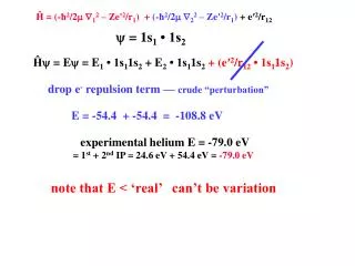
Ĥ = (-ħ2/212– Ze'2/r1) + (-ħ2/222 – Ze'2/r1) +e′2/r12 y= 1s1 • 1s2 Ĥy= Ey = E1 • 1s11s2 + E2 • 1s11s2+ (e′2/r12 • 1s11s2) drop e- repulsion term — crude “perturbation” E = -54.4 + -54.4 = -108.8 eV experimental helium E = -79.0 eV = 1st + 2nd IP = 24.6 eV + 54.4 eV = -79.0 eV note that E < ‘real’ can’t be variation
Approximation Methods ― Perturbation Ĥ = Ĥ0+ Ĥ' Ĥ0y= E0y E0= -108.8 eV y= 1s(1) 1s(2) = (1/p)(1/a)3 exp(-2r/a) <E'> = 0 y Ĥ ydt <E′> = yĤ‘ydt = y e2/(4peor12) ydt = 34.0 eV <E> = <E>˚ + <E′> = -108.8 + 34.0 = -74.8 eV Helium: experimental E = -79.0 eV Note that this value is greater than the actual E by 5.3%.
‘Effective’ Nuclear Charge, Z′ replaces Z accounts for ‘shielding’ of nuclear attraction due to other e- 1s(1) = (p)-1/2(Z′/a)3/2 exp(-Z′r/a) Approximation Methods ― Variation Variation theory often introduces a term in the wavefunction, f, that can be continuously adjusted in numerous iterations until the minimum energy (best) is obtained. Variation: = N • 1s(1) 1s(2) 1s(1) = (p)-1/2 (Z/a)3/2 exp(- Zr/a) see example 12.11 on page 396 Adjust Z′ (1.6875) to minimize <E> to -77.5 eV the error is now down to 1.9%
Use H-like wave functions to represent each electron in the He atom. = N • 1s(1) 1s(2) 1s(1) = (p)-1/2(Z′/a)3/2 exp(-Z′r/a) This variational wave function only accounts for 3 q#sfor each electron: n, ℓ, mℓ. It does not account for spin which is not evident in basic QM, but added as the 6thpostulate based on Dirac’s Relativistic QM. spin angular momentum quantum # (s) fermions ― s = ½ & ms = ± ½
2-1/2[(1) (2) + (1) (2)] 2-1/2[(1) (2) - (1) (2)] Pauli Exclusion Principle We must now introduce the spin function to our He wave function (1) (2) (1) (2) (1) (2) (2) (1) Can’t distinguish electrons – use linear combination totalspin = =1s(1)a 1s(2)a +1 =1s(1)1s(2) • 2-1/2[(1) (2) + (1) (2)] 0 =1s(1)1s(2) • 2-1/2[(1) (2) - (1) (2)] 0 =1s(1)b 1s(2)b -1 Angular momenta of charged particles can be distinguished using magnetic fields. Experiments show He to have spin = 0.
Pauli Exclusion Principle If 2 electron wave function.... must be antisymmetric with respect to interchange of electrons. If the electrons are exchanged the wavefunction must change signs. =1s(1)1s(2) • 2-1/2[(1) (2) + (1) (2)] =1s(1)1s(2) • 2-1/2[(1) (2) - (1) (2)] = spatial •spin functions = sym •anti-sym =1s(1)1s(2) • 2-1/2[(1) (2) - (1) (2)] 12.10 Show that this is antisymmetric with respect to electron exchange
Pauli Exclusion Principle 12.10 Show that this is antisymmetric with respect to electron exchange =1s(2)1s(1) • 2-1/2[(2) (1) - (2) (1)] = ….. = spatial •spin functions = sym •anti-sym =1s(1)1s(2) • - 2-1/2[-(2) (1) + (2) (1)] = ….. =1s(1)1s(2) • 2-1/2[(1) (2) - (1) (2)] =1s(1)1s(2) • - 2-1/2[-b(1) a(2) + a(1) b(2)] = ….. =1s(1)1s(2) • - 2-1/2[(1) (2) - (1) (2)] = ….. =-{1s(1)1s(2) • 2-1/2[(1) (2) - (1) (2)]} = …..
represented in matrix form ....... 1s(1) (1) 1s(1) (1) 1s(2) (2) 1s(2) (2) He,gs = 2-1/2 He,gs =1s(1) 1s(2) 2-1/2[(1) (2) - (1) (2)] Multi-electron wavefunctions can be represented as n x n matrices where n is the number of electrons in the atom (which is also = to the number of columns and rows in the matrix. The renormalization constant is n!-1/2 . + 1s 1s e- #1 e- #2 - Cross-multiplying the matrix will give you the determinant of the matrix (called the Slater determinant) which is also the ground state wavefunction for the atom.
1s(1) (1) 1s(1) a(1) 1s(2) (2) 1s(2) a(2) He,gs≠ 2-1/2 = 0 If any column or row of the matrix is identical, the determinant is 0. Therefore the wavefunction would also have to be 0, which is not valid. Lithium atom matrix Pauli Exclusion Principle ― antisymmetric regarding exchange of electrons no more than two electrons in an orbital no two electrons can have the same set of 4 quantum #s
^ Satisfy F fi = eifi Hartree–Fock Wave Functions (linear variation theory p398) Variational method using non-hydrogen-like wave functions that retain ‘orbital’ analogy Hartree-Fock Operator – equivalent to Ĥ i = quantum number related to orbital ei = energy of ith state fi = Hartree-Fockvariational function for ith state Hartree-Fock treatment of He ― <E> = -77.9 eV Hydrogen-like f = -77.5 eV Real He atom = -79.0 eV HF neglects instantaneous correlations in motions of electrons – improved on by configuration interactions (CI)
^ Satisfy F fi = eifi Hartree–Fock Wave Functions (linear variation theory p398) Variational method using non-hydrogen-like wave functions that retain ‘orbital’ analogy Hartree-Fock Operator – equivalent to Ĥ i = quantum number related to orbital ei = energy of ith state fi = Hartree-Fockvariational function for ith state Hartree-Fock treatment of He ― <E> = -77.9 eV Hydrogen-like f = -77.5 eV Real He atom = -79.0 eV HF neglects instantaneous correlations in motions of electrons – improved on by configuration interactions (CI)
Li,gs 1s(1) (1) 1s(1) (1) 2s(1) (1) 1s(2) (2) 1s(2) (2) 2s(2) (2) 1s(3) (3) 1s(3) (3) 2s(3) (3) 6-1/2 The Slater determinant for Li will have 6 terms Note that putting 1s again in the third column forces two identical columns For atoms with increased numbers of electrons it is the total energy that determines the filling order not the individual energy of the H-like orbital. This is why the 4s orbital is lower in energy than 3d and that there are many ‘exceptions’ to the filling rules. Once again the paired concepts of penetration and shielding provides a rationale for these energy changes (see fig. 12.5 on p385)
Li,gs 1s(1) (1) 1s(1) (1) 2s(1) (1) 1s(2) (2) 1s(2) (2) 2s(2) (2) 1s(3) (3) 1s(3) (3) 2s(3) (3) 6-1/2 E = -Z2e4m/(8eo2h2n2) 12.8
Li,gs 1s(1) (1) 1s(1) (1) 2s(1) (1) 1s(2) (2) 1s(2) (2) 2s(2) (2) 1s(3) (3) 1s(3) (3) 2s(3) (3) 6-1/2 The number of terms in the wavefunction is n! where n is the # of electrons in the atom. 12.14
Helium excited states 1s 2s and the Pauli exclusion principle … 2-1/2[1s(1) 2s(2)+1s(2) 2s(1)]2-1/2[(1) (2) - (1) (2)] 2-1/2[1s(1) 2s(2) - 1s(2) 2s(1)]2-1/2[(1) (2) + (1) (2)] (1) (2) b(1) b(2) L = Sℓ (for all e-) Total Orbital Angular Momentum gs: ℓ(1) = 0 & ℓ(2) = 0; L = 0 same for 1s 2s es 1s 2p excited states: L = 0 + 1 = 1 Total Orbital Angular Momentum = [L(L + 1)]1/2ħ
Spectroscopic Term Symbols for es L =symbol e.g. 1S0 = singlet ground state 1S1 = 1st singlet excited state electrons still have opposite spins 3S = triplet excited state electrons still have like spins 0 1 2 3 S P D F 1s 2s 1s 2p 1s 3d 2-1/2[1s(1) 2s(2) - 1s(2) 2s(1)]2-1/2[(1) (2) + (1) (2)] (1) (2) b(1) b(2) Total Spin Angular Momentum S = |S ms | (for all e-) gs: ms = ½ & ms = - ½ ; S = 0 if S = 0 then 2S + 1 = 1 (singlet) paired if S = 1 then 2S + 1 = 3 (triplet) unpaired multiplicity = 2S + 1
Linear variation theory (p-398) Variation functions are often obtained by taking a basis set of functions, yi, each of which meets the requirements for any acceptable wavefunction, y, and may be related to multiple states of some related or model system. Each of the basis set of functions is multiplied by an adjustable constant such that the overall variationalwavefunctionf is …… f = Sici • yi The constants (ci) fulfill three separate requirements: Combined, they serve to normalize the variational function. Individually they act as weighting factors that indicate the magnitude of the contribution for each function in the basis set. They become the adjustable factors used to minimize the system energy to give the best variational function such that ….. dE/dc1 = dE/dc2 = …. dE/dci = 0 This minimization process leads to the best value for the energy of the system, as well as the values for the coefficient for each basis set function.
Linear variation theory f = Sici • yi Using a general example that has only two basis set functions …… f = c1y1 + c2y2 Set up the expression for <E> …… ∫ f*Ĥ fdt ≥ E ∫ f*fdt Only needed if f is un-normalized function ∫ (c1y1 + c2y2 )*Ĥ (c1y1 + c2y2 )dt ≥ E ∫ (c1y1 + c2y2 )* (c1y1 + c2y2 )dt The solution involves (see 12.28 on p398) energy integral …. H11, H22, H12/H21 overlap integrals ... S11, S22, S12/S21 e.g. H11= ∫ y1*Ĥy1dt etc. e.g. S12 = S21 = ∫ y1*y2dt etc.
H11 – ES11 H12 – ES12 H21 – ES21 H22 – ES22 = 0 Linear variation theory f = Sici • yi Using a general example that has only two basis set functions …… f = c1y1 + c2y2 Set up the expression for <E> …… = ∫ f*Ĥ fdt ≥ E ∫ f*fdt Matrix solution for <E> …… e.g. H11= ∫ y1*Ĥy1dt etc. e.g. S12 = S21 = ∫ y1*y2dt etc.
H11 – ES11 H12 – ES12 H21 – ES21 H22 – ES22 = 0 Using a general example that has only two basis set functions …… f = c1y1 + c2y2 Example 12.12 The determinant for this matrix gives a binomial function in E, which can be solved to give 2 possible values … E1 and E2. Then solve for c1 and c2 by …… c1/c2 = - (H12 – ES12)/(H11 – ES11) and … c1/c2 = - (H22 – ES22)/(H21 – ES21) These apply to both E1 and E2. If y1 and y2 are orthonormal, then …. c12 + c22 = 1 See figures 12.9 and 12.10 on page 402
f = c1y1 + c2y2 and f* = c1y1 - c2y2 Example 12.12 2 orthonormalwavefunctions H11 = -15, H22 = -4, H12 = H21 = -1 Find E and E* and the coefficients of each variationalwavefunction -15 – E -1 -1 -4 – E H11 – ES11 H12 – ES12 H21 – ES21 H22 – ES22 = 0 = 0 E2 +19E + 59 = 0 & E = -15.09 & -3.91 c1/c2 = - (H12 – ES12)/(H11 – ES11) c1/c2 = - (H22 – ES22)/(H21 – ES21) • f = 0.996y1 + 0.0896y2 and • f* = -.0896y1 + 0.996y2
Molecular Properties What data would you want to know to understand the properties of a diatomic molecule? Bond distance Bond energy Dipole moment What additional information would you want to extend this to a polyatomic molecule? Molecular geometry or bond angles How did General Chemistry guide you in predicting this data?
Molecular Properties Geometry ― bond lengths bond angles VSEPR sp, sp2, sp3 hybrids “A hybrid AO is a LCAO from same atom” “The purpose of hybrid AOs is to rationalize the observed geometry on a molecule” Stability and reactivity ― bond energies dipole moments (e-distribution) Empirical treatment Tables of ‘averaged’ bond energies The Pauling electronegativity scale Theoretical Molecular Methods Empirical ― uses ‘averaged’ experimental data Ab initio ― uses QM theory only ‘from scratch’ Semi-empirical ― uses ‘averaged’empirical data as a starting point and makes adjustments using theoretical QM methods.
Using Empirical Values (e.gbond length/energy) accumulate experimental data from many compounds. find average values for the same type of bond. establish a table with these ‘averaged’ values. assume value is the same regardless of the larger molecular context.
Dipole Moments & Electronegativity CH2O Geometry In MO theory the charge on each atom is related to the probability of finding the electron near that nucleus, which is related to the coefficient of the AO in the MO
Ĥe = Ke+ VNN + VNe + Vee Ĥ = KN + Ke + VNN + VNe + Vee ĤN= KN + VN VN = Ee nucleus is slow & electron fast 1. electron “sees” nucleus as stationary 2. nucleus “sees” electrons as time- averaged cloud ĤNyN = (KNyN + EeyN) = ENyN QM treatment of molecules ― Hamiltonian Born-Oppenheimer Approximation ― = eN Electrical Energy at fixed R ― <E> = ∫eĤe
H2+ Molecular Ion Basis set = 1s1 and 1s2 LCAO = f1 = c1(1s1 + 1s2) f f2 = c2(1s1 - 1s2) f* ∫ f12dt = c12 ∫(1s1 + 1s2) 2 = 1 = c12(∫ 1s12 + ∫2 1s11s2 + ∫1s22) = c12 (1 + ∫2 1s11s2 + 1) = c12 (2 + 2∫1s11s2) = c12 (2 + 2S) = 1 c1 = 1/(2 + 2S)½
H2+ Molecular Ion true Re 1.06 1.32 1.07 Å De2.8 1.8 2.35 eV f = C (1s1 + 1s2) òf*Ĥfdt òf*fdt <E> = C2•ò (1s1 + 1s2) Ĥ (1s1 + 1s2) dt = ò1s1Ĥ1s1 + ò1s2Ĥ1s2 + 2ò1s1Ĥ1s2 ò (1s1 + 1s2)2dt ò 1s12 + ò 1s22 + 2ò1s11s2 = H11 + H22 + H12 + H21 = 2(H11 + H12) = H11 + H12 2 + 2S12 1 + S12 <E>′ = H22 - H12 1 - S12 s* -13.6 eV H2 H1 ↑ -15.4 eV s s bond ― f is symmetrical about bonding axis
12.36 E1 should reach minimum at 1.32?
2AO’s give 2 MO’s - one bonding & one anti-bonding 0.9 eV -13.6 eV ' -19.0 eV • <E>= H11 + H12 1 + S12 <E>′ = H22 - H12 1 - S12 Ee s* H2 H1 s r
Bond Types bond types , , , etc. arise from m quantum # & orbital angular momentum along z axis (= mħ) (z axis = bonding axis) s - s; s - pz; pz - pz px - px or py - py requires d orbitals
2nd period diatomic molecules s* p* 2px 2py 2pz 2s 2pz 2py 2px 2s s p s* s AO #2 AO #1 MO
Diatomic MOs More complete treatments make MOs from larger AO sets. AOs used must be same type s vs. p. mix s and pz as s px and py remain as p AOs used must have same symmetry. g vs. u
Homonuclear Diatomic molecules H2(g1s)2 He2 (g1s)2 (u*1s)2 C2 (g1s)2 (u*1s)2 (g2s)2 (u*2s)2 (u2p)4(g2p)0(g*2p)0 N2 (g1s)2 (u*1s)2 (g2s)2 (u*2s)2 (u2p)4(g2p)2(g*2p)0 O2 (g1s)2 (u*1s)2 (g2s)2 (u*2s)2 (g2p)2(u2p)4(g*2p)2 F2(g1s)2 (u*1s)2 (g2s)2 (u*2s)2 (g2p)2(u2p)4(g*2p)4
Diatomic MOs More complete treatments make MOs from larger AO sets. AOs used must be same type s vs. p. mix s and pzas s px and py remain as p AOs used must have same symmetry. g vs. u
Semi-empirical treatment of N2 from Spartan (AM1) -14.5 eV MO: 1 2 3 4 5 Eigenvalues:-1.52116 -0.78755 -0.59504 -0.59504 -0.52636 (ev): -41.39299 -21.43028 -16.19199 -16.19199 -14.32295 Sg+ Su+ ??? ??? Sg+ 1 N2 S 0.62096 0.64963 0.00000 0.00000 0.33825 2 N2 PX 0.00000 0.00000 0.63756 -0.30581 0.00000 3 N2 PY 0.00000 0.00000 -0.30581 -0.63756 0.00000 4 N2 PZ 0.33825 -0.27924 0.00000 0.00000 -0.62096 5 N1 S 0.62096 -0.64963 0.00000 0.00000 0.33825 6 N1 PX 0.00000 0.00000 0.63756 -0.30581 0.00000 7 N1 PY 0.00000 0.00000 -0.30581 -0.63756 0.00000 8 N1 PZ-0.33825 -0.27924 0.00000 0.00000 0.62096 MO: 6 7 8 Eigenvalues: 0.03684 0.03684 0.22165 (ev): 1.00254 1.00254 6.03130 ??? ??? Su+ 1 N2 S 0.00000 0.00000 0.27924 2 N2 PX -0.66629 0.23675 0.00000 3 N2 PY 0.23675 0.66629 0.00000 4 N2 PZ 0.00000 0.00000 0.64963 5 N1 S 0.00000 0.00000 -0.27924 6 N1 PX 0.66629 -0.23675 0.00000 7 N1 PY -0.23675 -0.66629 0.00000 8 N1 PZ 0.00000 0.00000 0.64963
Semi-empirical treatment of N2 from Spartan (AM1) -14.5 eV Heat of Formation: 46.7 kJ/mol 8) +6.03eV su 0.279 N22s + 0.650 N22pz - 0.279 N12s + 0.650 N12pz : 7) +1.00 eVp0.237 N22px + 0.666 N22py - 0.237 N12px - 0.666 N12py : 6) +1.00 eVp - 0.666 N22px + 0.237 N22py + 0.666 N12px - 0.237 N12py : 5) -14.3 eVsg 0.338 N22s - 0.621 N22pz + 0.338 N12s + 0.621 N12pz : 4) -16.2 eVp - 0.306 N22px - 0.638 N22py - 0.306 N12px - 0.638 N12py : 3) -16.2 eVp0.638 N22px - 0.306 N22py + 0.638 N12px - 0.306 N12py : 2) -21.4 eVsu0.650 N22s - 0.279 N22pz - 0.650 N12s – 0.279 N12pz : 1) -41.4 eVsg0.621 N22s + 0.338 N22pz + 0.621 N12s – 0.338 N12pz :
Semi-empirical treatment of O2 from Spartan (AM1) -13.6 eV MO: 1 2 3 4 5 Eigenval : -1.69510 -1.12412 -0.71524 -0.70967 -0.69421 (ev): -46.12594 -30.58885 -19.46255 -19.31098 -18.89045 Sg+ Su+ ??? Sg+ ??? 1 O2 S -0.61708 -0.67817 0.00000 -0.34528 0.00000 2 O2 PX 0.00000 0.00000 0.21578 0.00000 0.67338 3 O2 PY 0.00000 0.00000 0.67338 0.00000 -0.21578 4 O2 PZ -0.34528 0.20020 0.00000 0.61708 0.00000 5 O1 S -0.61708 0.67817 0.00000 -0.34528 0.00000 6 O1 PX 0.00000 0.00000 0.21578 0.00000 0.67338 7 O1 PY 0.00000 0.00000 0.67338 0.00000 -0.21578 8 O1 PZ 0.34528 0.20020 0.00000 -0.61708 0.00000 MO: 6 7 8 Eigenvalues: -0.38542 -0.01916 0.23853 (ev): -10.48773 -0.52126 6.49061 ??? ??? Su+ 1 O2 S 0.00000 0.00000 0.20020 2 O2 PX -0.21578 -0.67338 0.00000 3 O2 PY -0.67338 0.21578 0.00000 4 O2 PZ 0.00000 0.00000 0.67817 5 O1 S 0.00000 0.00000 -0.20020 6 O1 PX 0.21578 0.67338 0.00000 7 O1 PY 0.67338 -0.21578 0.00000 8 O1 PZ 0.00000 0.00000 0.67817
Semi-empirical treatment of O2 from Spartan (AM1) -13.6 eV 8) +6.49 eVsu 0.200 O22s + 0.678 O22pz - 0.200 O12s + 0.678 O12pz : 7) -0.52 eVp - 0.673 O22px + 0.216 O22py + 0.673 O12px - 0.216 O12py : 6) -10.5 eVp - 0.216 O22px - 0.673 O22py + 0.216 O12px + 0.673 O12py : 5) -18.9 eVp0.673 O22px - 0.216 O22py + 0.673 O12px - 0.216 O12py : 4) -19.3 eVsg - 0.345 O22s + 0.617 O22pz - 0.617 O12s - 0.345 O12pz : 3) -19.5 eVp0.216 O22px + 0.673 O22py + 0.216 O12px - 0.673 O12py : 2) -30.6 eVsu - 0.678 O22s - 0.200 O22pz + 0.678 O12s + 0.200 O12pz : 1) -46.1 eVsg - 0.617 O22s - 0.345 O22pz - 617 O12s + 0.345 O12pz :
Heteronuclear Diatomic molecules HF 1s2 2s2 3s2 (1p22p2)4s0 Basis set s = H1s (-13.6 eV), F1s (??), F2s (-40.2 eV?), F2pz (-18.6 eV) p = F2px and F2py (-18.6 eV) One simpler treatment of HF is given in Atkins on page 428 gives the following results.... 4s = 0.98 (H1s) - 0.19(F2pz) -13.4 eV px = py = F2px and F2py -18.6 eV 3s = 0.19(H1s) + 0.98(F2pz) -18.8 eV 2s = F2s ~ -40.2 eV 1s = F1s << -40.2 eV A more complicated system might mix all s type AOs in the following fashion.... 4s = ??? px = py = F2px and F2py 3s = -0.023(F1s) -0.411(F2s) +0.711(F2pz) +0.516(H1s) 2s = -0.018(F1s) +0.914(F2s) +0.090(F2pz) +0.154(H1s) 1s = 1.000(F1s) +0.012(F2s) +0.002(F2pz) -0.003(H1s)
HF 1s22s23s2(1p22p2)4s0 Semi-empirical treatment of HF from Spartan (AM1) MO: 1 2 3 4 5 Eigenvalues:-1.82822 -0.63290 -0.51768 -0.51768 0.24632 (ev): -49.74849 -17.22198 -14.08688 -14.08688 6.70261 A1 A1 ??? ??? A1 1 H2 S 0.37583 -0.46288 0.00000 0.00000 0.80281 2 F1 S 0.91940 0.29466 0.00000 0.00000 -0.26052 3 F1 PX 0.00000 0.00000 -0.78600 0.61823 0.00000 4 F1 PY 0.00000 0.00000 0.61823 0.78600 0.00000 5 F1 PZ -0.11597 0.83601 0.00000 0.00000 0.53631 H1s F2p F2s One simpler treatment of HF is given in Atkins on page 428 gives the following results.... 4s = 0.98 (H1s) - 0.19(F2pz) -13.4 eV px = py = F2px and F2py -18.6 eV 3s = 0.19(H1s) + 0.98(F2pz) -18.8 eV 2s = F2s ~ -40.2 eV 1s = F1s << -40.2 eV