Download

1 / 34
350 likes | 546 Vues
Math 6700 Presentation Qualitative Ordinary Differential Equations Laura Lowe and Laura Singletary December 15, 2009. The Collapse of Tacoma Narrows Bridge: The Ordinary Differential Equations Surrounding the Bridge Known as Galloping Gertie. The Tacoma Narrows Bridge.

E N D
Math 6700 Presentation Qualitative Ordinary Differential Equations Laura Lowe and Laura Singletary December 15, 2009 The Collapse of Tacoma Narrows Bridge: The Ordinary Differential Equations Surrounding the Bridge Known as Galloping Gertie
The Tacoma Narrows Bridge Construction on the Tacoma Narrows Bridge began in November 1938 and was completed on July 1, 1940. The structure of the bridge was characterized by lightness, grace, and flexibility. The completion of the bridge was heralded as “a triumph of man's ingenuity and perseverance”
Galloping Gertie During construction, the roadbed flexed or displayed vertical oscillations This raised questions about the bridge’s stability. A light wind of 4 mph could cause these oscillations Additional engineers were contracted to “fix” these oscillations People came from hundreds of miles away to experience driving on Galloping Gertie
Galloping Gertie: On the fateful morning, the center span experienced vertical oscillations of 3 to 5 ft under wind speeds of 42 mph The Bridge was closed by 10:00 AM on November 7, 1940
Galloping Gertie: The motion changed to a two-wave torsional motion causing the roadbed to tilt as much as 45 degrees This motion continued for 30 minutes before a panel from the center span broke off
Galloping Gertie’s Gallop By 11:00 am, the center span of the Tacoma Narrows Bridge had fallen into Puget Sound
The Collapse: Reporters, engineers, and passersby witnessed the collapse at 11:00 AM The only fatality was a dog abandoned in a car on the bridge Eventually called the “Pearl Harbor of Engineering”
Eyewitness Report by Leonard Coatsworth : "Just as I drove past the towers, the bridge began to sway violently from side to side. Before I realized it, the tilt became so violent that I lost control of the car... I jammed on the brakes and got out, only to be thrown onto my face against the curb. "Around me I could hear concrete cracking. I started to get my dog Tubby, but was thrown again before I could reach the car. The car itself began to slide from side to side of the roadway. "On hands and knees most of the time, I crawled 500 yards or more to the towers... My breath was coming in gasps; my knees were raw and bleeding, my hands bruised and swollen from gripping the concrete curb... Toward the last, I risked rising to my feet and running a few yards at a time... Safely back at the toll plaza, I saw the bridge in its final collapse and saw my car plunge into the Narrows."
"A few minutes later I saw a side girder bulge out on the Gig Harbor side, due to a failure, but though the bridge was buckling up at an angle of 45 degrees the concrete didn't break up. Even then, I thought the bridge would be able to fight it out. Looking toward the Gig Harbor end, I saw the suspenders -- vertical steel cables -- snap off and a whole section of the bridge caved in. The main cable over that part of the bridge, freed of its weight, tightened like a bow string, flinging suspenders into the air like so many fish lines. I realized the rest of the main span of the bridge was going so I started for the Tacoma end."
Purpose: Our project plans to explore the events surrounding this catastrophe: We will explore a complex model proposed by Dr. P. J. McKenna that takes into account the potential and kinetic energy involved with the oscillations of the Bridge.
Mathematical Models Vertical Kinetic Energy: Torsional Kinetic Energy: Total Kinetic Energy:
Mathematical Models Vertical Potential Energy: Torsional Potential Energy: Total Potential Energy:
L= KETotal – PE Total Mathematical Models Lagrangian Equations:
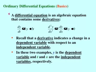
Mathematical Models After a bunch of math… is the forcing term are the dampening terms
Mathematical Models Assuming the cables never lose tension, let and Then simplify and we get:
Mathematical Models • The mass of the center span was approximately 2500 kg/ft, and 12m wide. • The bridge deflected approximately 0.5m per 100kg/ft. Hooke’s Law: F = -kx So k ≈ 1000
Mathematical Models Let Then, since the bridge oscillated at a frequency of 12-14 cycles per minute, And let
Mathematical Models Put it all together and we get:
Mathematical Models System of ODE’s:
Mathematical Models In 1940, the technology was not available to solve a non-linear system. Instead, the engineers of the time used a linearized ODE believing that would give them the information they needed. In the following slides we will compare these two ODE’s.
Linear vs. Non-linear Linear model with initial conditions and (large push)
Linear vs. Non-Linear Non-linear model with initial conditions and (large push)
Linear vs. Non-linear Linear model with initial conditions and (large push)
Linear vs. Non-linear Non-linear model with initial conditions and (large push)
Linear vs. Non-linear Non-linear model with initial conditions and (large push)
Linear vs. Non-linear Non-linear model with initial conditions and (large push)
Unforced Model The unforced, non-linear model with
Conclusions Here we focused on the torsional motion of the bridge with specific emphasis on the forcing term. We assumed the cables did not lose tension and that the torsion was symmetric and independent from the vertical motion.
Areas of Further Research Broughton Bridge Angers Bridge Millennium Bridge
References Hobbs, R. S. (2006). Catastrophe to triumph: Bridges of the Tacoma Narrows. Pullman, WA: Washington State University Press. McKenna, P. J. (1999). Large torsional oscillations in suspension bridges revisited: Fixing an old approximation. The American Mathematical Monthly, 106, 1-18.