Download
1 / 149
1.55k likes | 2.01k Vues
Agricultural Land use Pattern - Von Thunen Model. Introduction. Von Thunen Model Explain the agricultural landuse at a given location Put the emphasis on economic factors rather than treat physical factors as the main forces Distance from market. Aim of Von Thunen Model.

E N D
Introduction • Von Thunen Model • Explain the agricultural landuse at a given location • Put the emphasis on economic factors rather than treat physical factors as the main forces • Distance from market
Aim of Von Thunen Model • Showing how and why agricultural landuse varies with the distance from the market • Economic rent net return from a unit of land
A. Assumptions of the model A. Explicit assumptions B. Implicit assumptions
A. Explicit assumptions • 1. An isolated state • 2. Centrally located market • the sole urban market • 3. Isotropic plain • production and transport costs were the same everywhere • 4. Uniform transportation and transport costs • Only one form of transport (Wagon) • Increase distance, increase transport cost • 5. Farmers are economic men and aim at maximizing profits • 6. Same market price
B. Implicit assumptions • 1. Land use competition under a capitalistic economy • 2. Economic rent is the determining factor • 3. Productivity could be raised • 4. Steepness of an economic rent curves are governed by the degree of perishability of farm produce and the relative ease of transporting\
B. Implicit assumptions • 5. Growing of temperate area crops • 6. No catastrophic event • 7. No chance factor • 8. All parties are price-takers under perfect competition
Why did Von Thunen establish so many assumptions? • Simplify the complex reality
B. Concepts of the models Economic Rent Distance decay mechanism
A. Economic rent • Net return • Highest bid rent ability • Displace all others • Exercise
A. Economic rent • Net return • = 1. Market price – 2. Production cost – 3. Transport cost • 1. Farmers got the same price (revenue) for their crops • 2. Production cost = constant • 3. Transport cost increase with distance • = Net return decreases with increasing distance from the market
Formula for locational rent • EXERCISE!!!
Economic rent --- Conclusion • Different crops have different location rent distribution patterns (bit rent curves) • Different crops compete with each other’s farmland • Concentric land use pattern was formed
B. Distance decay mechanism • Locational rent decreasing with increasing distance from market
Describe how the net profit from wheat growing varies with distance from the urban market. • Net return decreases with increasing distance from market • At the market, transport cost contributes nothing to total cost. As there is no transport cost incurred, net return at market • = market price – production cost • = $40 - $10 • = $30
At point 180km from the market, net return = $0, farmers would not produce because there is no incentive. • Beyond point 180km from market, a loss will be incurred in producing any crops. Thus, farmers would not produce any crops.
Economic Rent +Distance Decay Mechanism Examination Practice
Starting point = number of unit x (market price – production cost) (NO TRANSPORT COST) Ending point = The distance that market price = transport cost
Locational rent per unit: Market price – production cost 12 – 3.5 = 8.5 Transport cost per unit $7 / 35km = $8.5 / ?km
Starting point = number of unit x (market price – production cost) (NO TRANSPORT COST) Ending point = The distance that market price = transport cost
Theory of the model • A. Intensity Theory • Land use intensity declines with distance from the market. • More intensive farming activities tend to locate near the market. • Less intensive farming activities tend to locate far away from the market.
B. Crop Theory • Crops with the highest economic rent will be grown. This concept applies to any location.
1. Free cash cropping (Market Gardening) • Horticulture (vegetables and fruit) and dairying • Perishable as close as possible to market • Low speed of transport • No refrigeration • Require milk and vegetable in city + price are high higher economic rent • Intensive labour input, multi-cropping, heavy fertilizing • Horse provide motive power
2. Forestry (firewood) • Great demand of wood • Bulky (heavy and big) • High transport cost = economic rent decrease fast with increase of distance
3. Crop Alternation System (Six-year crop rotation) • Crop without fallowing • 6-year crop rotation • 2 years of rye (黑麥)+ 1 year potato + 1 year barley (大麥)+ 1 year clover (三葉草)+ 1 year vetch (巢菜) • Soil conserved by rotation
4. Improved System (Seven-year crop rotation) • Zone of farming, fallow and pasture • Less intensive • 7-year crop rotation • Rye = 1/7 • Barley = 1/7 • Oats = 1/7 • Pasture = 3/7 • Fallow = 1/7 • Prodcut: rye, butter, cheese live animals
5. Three-field system • 1/3 pasture • 1/3 field crop • 1/3 fallow • Rotation
6. Stock Farming • 400km away • Extensive grazing activities
In 1826, Von Thunen noted the followings: • 1. Production costs are nothing simple • 2. There is no large town that does not lie on a navigable river or canal • 3. Competing markets • 4. Different places possess different physical factors • 5. Farmers do not maximize profits
The modified patterns • 1. Additional of a navigable river • Navigable river with lower transport cost
2. A new railway connecting the city and its fringe area • 2 or more kinds of transports • The actual cost = distance traveled by each method • Not physical distance, but economic distance
4. Localized fertile soil or localized infertile soil/ hilly terrain
5. Variation in farmers’ amount of information and their abilities to use the information
Market cost and Production cost • 1. Increase in market price and decrease in production cost lead to an increase in profits expansion of extensive margin • 2. Decrease in market cost and increase in production cost lead to an decrease in profits contraction of extensive margin
Transport cost • 3. Transport cost has little effect on farms located near the market • 4. Increase in transport cost • contraction of the concentric ring because farms near the extensive margin become unprofitable • 5. Decrease in transport cost • extensive margin expand
Summary table of the effects of change in market price, production cost and transport cost
Merits A. show the importance of economic factors B. show how does distance affect intensity C. showed the change of agricultural land use pattern (by transport cost) D. first theory to show the spatial distribution of agricultural activities