Download

1 / 19
190 likes | 205 Vues
Learn about linear programming, dynamic programming, and systems simulation as powerful analytical techniques for analyzing farming systems.

E N D
Farm Business Management: The Fundamentals of Good Practice Peter L. Nuthall
Chapter 15 Introducing Further Methods of Farm Systems Analysis
Discover the form of the powerful analytical technique known as linear programming (LP). Learn how to relate LP to production economics. Become familiar with the assumptions embodied in the LP model of a farm. Understand Bellman’s dynamic programming (DP) and its representation of dynamic (time-dependent), non-certainty full decision problems. Consider the assumptions in the DP model, and understand the solving difficulties due to the extensive nature of DP model sizes. Learn about systems simulation and the process of creating, and using, these ‘free form’ models.
Use of Sophisticated Techniques for Analysing Farming Systems Farmers mainly improve their farming system by making small marginal changes from time to time. Consultants, similarly, mainly recommend marginal changes be made from an existing system. Marginal changes are made through time as improvements are recognized and conditions change. Techniques used are mainly budgeting, benchmarking, survey results. Optimal systems: to consider possible marginal changes it is useful to have information on likely optimal systems. To determine optimal systems, without regard to change limitations, analytical systems to consider are linear programming, dynamic programming and systems simulation.
Linear Programming: The Farm Decision Problem To find a farm system that maximizes the objectives subject to the limitations imposed by the resources available. That is, find xj values that maximize Z. Objective Z = C1x1 + C2x2 + … + Cnxn where Cj = net revenue per unit of the jth production activity xj=level of production of the jth production activity n = the maximum number of production activities Subject to b1 ≥ r1,1x1 + r1,2x2 + … + r1,nxn,…through to bm≥ rm,1x1 + rm,2x2 + … + rm,nxn where b1= quantity of the first resource restricting production; there are m restricting resources; ri,j= the per unit requirement of the xj activity for the mth resource; xj ≥ 0 all j.
Linear Programming: Graphical Representation 1 The feasible area (2 variable case and 2 constraints): Shaded area: combination of variables that are feasible with respect to resources. Reality is multi-dimensional, but follows the same principles.
Linear Programming: Finding the Optimal Solution Using a Graph Optimal point must be on the feasible boundary if production is to be profitable. Solution on boundary because no other higher feasible point(s): shows stability; method: matrix algebra (simplex method); iterative: start at origin and move on boundary.
Linear Programming: Assumptions Objective: can be expressed using a linear function with no interactions (though linear segmentation allows decreasing returns). Input/output coefficients: are fixed (but can have segmented increases) and enter linearly. Divisibility: variables are infinitely divisible (but can have integer systems imposed on some, e.g. tractor purchase). Certainty: variables and coefficients are known with certainty (but special modifications are possible that allow for probabilities). Finiteness: a finite limit to variable and resource numbers exists.
Linear Programming: The Solution The solution provides more than just the optimal solution. Provides: alternative near optimal solutions (farm systems); values of all limiting resources, and the ranges over which they hold; price ranges over which the solution is optimal for variables in the solution, and for variables not in the solution (how much does their net revenue need to change before they become profitable?); ranges over which input/output ratios can vary without sub-optimality.
Dynamic Programming: The Basics Divides planning into distinct time periods that can vary in length (e.g. monthly). For given states of all farm resources at each time period, system works out optimal decisions. Solving occurs for each period in a step-by-step system, assuming knowledge exists about the value of each possible farm state (value for each state variable, e.g. working capital on hand) at period end (sometimes period beginning). Solve for each possible state the farm can be in for each period. Decisions relate to which state to move to from the existing state. Usually start at the last time period and work backwards. As proceed, know optimal decision for each state the farm might find itself in (uncertainty prevails).
Dynamic Programming: The Algebra of Solutions (1) Given Sj represents the state of the farm in period j, the state of the system is a function of the state in the previous period and the decisions taken (xj), thus Sj+ 1 = f(Sj,xj) and Rj= f(Sj,xj) where Rj is the return in period j.
Dynamic Programming: The Algebra of Solutions (2) Solving the period-by-period problem involves recognizing: (S ) = the $ return if an optimal policy (optimal decisions are made) is followed from stage j to the end of the process, assuming the process is in state iat the beginning of stage j. r(S ) = the return associated with moving from state i (the superscript on r) at the beginning of stage j to state i (the superscript on S) at the beginning of stage j + 1 (or endof stage j) (the return depends on the values of the decision variables necessary to give (S ) ). Thus, (S ) = max (r(S ) + fj + 1 (S) ion Si/j+1 (This is referred to as a recurrence relationship.) Thus, select the xj (decisions) that maximize this period-by-period return in total.
Dynamic Programming Assumptions and Problems Describable states exist using a quantification system with values for each resource and restriction impacting on the system. Connections between the period-by-period states result from the decisions made each period, and the relationships are definable through functions. Costs and returns relate to state movements and decisions, and are definable. There are no restrictions on the forms and types of the relationships impacting on state movements; assumptions are minimal. A defined standard solving algorithm does not exist; they are particular to each problem. With many state variables, the solving dimensionality can be overpowering, so restrict to small number of state variables and the values they can take on.
Dynamic Programming Lessons for Decision Making in General Problems are all multi-stage in reality. Uncertainty brings about a non-certain ending state (which is allowed for in DP). The solution (optimal decisions) to a DP problem provides the answer no matter which state the farm ends up in at the end of each period. The value of each resource (states) comes from the profit benefits. Decision problem solving only needs to look ahead a specific number of periods called the planning horizon. The horizon depends on how many periods to include so the first period solution is stable. Then re-solve each new period.
Systems Simulation: The Basics Involves developing an algebraic model for each specific decision problem. Structure is not limited to specific assumptions, but needs to be quantifiable. Solutions are obtained through repeated trials of the model. The complexity of the equations and relationship, and the need for repeated trials means SS is computer based. Budgeting is a very simple form of SS. In reality, all paper-based calculations are SS, including LP and DP. But only use the term SS for these free-form computer models. SS is expensive because each problem is set up specifically.
Systems Simulation: Operations Steps involve: define problem; collect input/output data: relationship equations (e.g. animal maintenance feed requirements, soil moisture relationships, plant growth with water); develop the structure of the problem (perhaps use a flow diagram); prepare the computer programs that represent the problem and its structure; run experiments for the problem; vary the decision variable; analyse the results to obtain a conclusion on optimal systems.
Systems Simulation: Monte Carlo Simulation Allow for non-certainty by either: using a series of historic values for all the parameters, or simulating a series of parameter values based on probabilities: draw many samples with the variable value selection based on their probabilities and correlations. Profit estimates: use the results of the physical simulations to calculate monetary outcomes. Optimal systems concluded through comparing profit estimates and/or calculating regression equations of profit using results.
Validation All models (LP, DP, SS, etc.) need verification and validation: do they sufficiently represent reality to provide useful conclusions? Methods include: comparing outputs with real farm outputs using the same input levels; comparisons with plot, experimental and other trials and data; seeking experts’ opinions of outputs for ranges of input levels; using only well-proven relationships on the assumption that taken together they must be realistic. Models are seldom ever perfect and can be constantly improved.
Name: First Surname Email: email@email.com