The Gibbs Factor
220 likes | 558 Vues
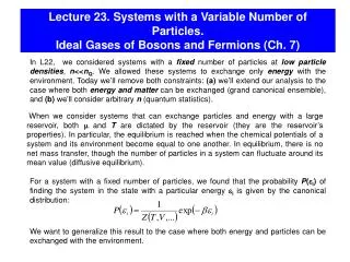
Lecture 23. Systems with a Variable Number of Particles. Ideal Gases of Bosons and Fermions (Ch. 7).

The Gibbs Factor
E N D
Presentation Transcript
Lecture 23. Systems with a Variable Number of Particles.Ideal Gases of Bosons and Fermions (Ch. 7) In L22, we considered systems with a fixed number of particles at low particle densities, n<<nQ. We allowed these systems to exchange only energy with the environment. Today we’ll remove both constraints: (a) we’ll extend our analysis to the case where both energy and matter can be exchanged (grand canonical ensemble), and (b) we’ll consider arbitrary n (quantum statistics). When we consider systems that can exchange particles and energy with a large reservoir, both and T are dictated by the reservoir (they are the reservoir’s properties). In particular, the equilibrium is reached when the chemical potentials of a system and its environment become equal to one another. In equilibrium, there is no net mass transfer, though the number of particles in a system can fluctuate around its mean value (diffusive equilibrium). For a system with a fixed number of particles, we found that the probability P(i) of finding the system in the state with a particular energy i is given by the canonical distribution: We want to generalize this result to the case where both energy and particles can be exchanged with the environment.
R S 2 1 The reservoir is now both a heat reservoir with the temperature T and a particle reservoir with The Gibbs Factor chemical potential . Because each single-particle energy level is populated from a particle reservoir independently of the other single particle levels, the role of the particle reservoir is to fix the mean number of particles. 1 and 2 - two microstates of the system (characterized by the spectrum and the number of particles in each energy level) Reservoir UR, NR, T, System E, N According to the fundamental assumption of thermodynamics, all the states of the combined (isolated) system “R+S” are equally probable. By specifying the microstate of the system i, we have reduced S to 1 and SS to 0. Thus, the probability of occurrence of a situation where the system is in state iis proportional to the number of states accessible to the reservoirR . The total multiplicity: neglect The changes U and N for the reservoir = -(the corresponding changes for the system). Gibbs factor =
The Grand Partition Function - proportional to the probability that the system in the state contains N particles and has energy E Gibbs factor = the probability that the system is in state with energy E and N particles: the grand partition function or the Gibbs sum is the index that refers to a specific microstate of the system, which is specified by the occupation numbersni: s {n1, n2,.....}. The summation consists of two parts: a sum over the particle number N and for each N, over all microscopic states i of a system with that number of particles. The systems in equilibrium with the reservoir that supplies both energy and particles constitute the grand canonical ensemble. In the absence of interactions between the particles, the energy levels Es of the system as a whole are determined by the energy levels of a single particle, i: i - the index that refers to a particular single-particle state. As with the canonical ensemble, it would be convenient to represent this sum as a product of independent terms, each term corresponds to the partition function of a single particle. However, this can be done only for ni<<1 (classical limit). In a more general case, this trick does not work: because of the quantum statistics, the values of the occupation numbers for different particles are not independent of each other.
From Particle States to Occupation Numbers Systems with a fixed number of particles in contact with the reservoir, occupancy ni<<1 Systems which can exchange both energy and particles with a reservoir, arbitrary occupancy ni 4 4 3 3 2 2 1 1 The energy was fluctuating, but the total number of particles was fixed. The role of the thermal reservoir was to fix the mean energy of each particle (i.e., each system). The identical systems in contact with the reservoir constitute the canonical ensemble. This approach works well for the high-temperature (classical) case, which corresponds to the occupation numbers <<1. When the occupation numbers are ~ 1, it is to our advantage to choose, instead of particles, a single quantum level as the system, with all particles that might occupy this state. Each energy level is considered as a sub-system in equilibrium with the reservoir, and each level is populated from a particle reservoir independently of the other levels.
From Particle States to Occupation Numbers (cont.) We will consider a system of identical non-interacting particles at the temperature T, i is the energy of a single particle in the i state, ni is the occupation number (the occupancy) for this state: The energy of the system in the state s {n1, n2, n3,.....} is: The grand partition function: The sum is taken over all possible occupancies and all states for each occupancy. The Gibbs sum depends on the single-particle spectrum (i), the chemical potential, the temperature, and the occupancy. The latter, in its tern, depends on the nature of particles that compose a system (fermions or bosons). Thus, in order to treat the ideall gas of quantum particles at not-so-small ni, we need the explicit formulae for ’s and nifor bosons and fermions.
“The Course Summary” (the Landau free energy) is a generalization of F=-kBT lnZ The grand potential • the appearance of μ as a variable, while computationally very convenient for the grand canonical ensemble, is not natural. Thermodynamic properties of systems are eventually measured with a given density of particles. However, in the grand canonical ensemble, quantities like pressure or N are given as functions of the “natural” variables T,V and μ. Thus, we need to use to eliminate μ in terms of T and n=N/V.
Bosons and Fermions One of the fundamental results of quantum mechanics is that all particles can be classified into two groups. Bosons: particles with zero or integer spin (in units of ħ). Examples: photons, all nuclei with even mass numbers. The wavefunction of a system of bosons is symmetric under the exchange of any pair of particles: (...,Qj,...Qi,..)= (...,Qi,...Qj,..). The number of bosons in a given state is unlimited. Fermions: particles with half-integer spin (e.g., electrons, all nuclei with odd mass numbers); the wavefunction of a system of fermions is anti-symmetric under the exchange of any pair of particles: (...,Qj,...Qi,..)= -(...,Qi,...Qj,..). The number of fermions in a given state is zeroor one (the Pauli exclusion principle). The Bose or Fermi character of composite objects: the composite objects that have even number of fermions are bosons and those containing an odd number of fermions are themselves fermions. (an atom of 3He = 2 electrons + 2 protons + 1 neutron hence 3He atom is a fermion) In general, if a neutral atom contains an odd # of neutrons then it is a fermion, and if it contains en even # of neutrons then it is a boson. The difference between fermions and bosons is specified by the possible values of ni: fermions:ni= 0 or 1 bosons: ni= 0, 1, 2, .....
Bosons & Fermions (cont.) Consider two non-interacting particles in a 1D box of length L. The total energy is given by The Table shows all possible states for the system with the total energy
The Partition Function of an Ideal Fermi Gas Let’s consider a system that consists of just one singlestate of energy i. The total energy of this state: ni i. The probability of this state to be occupied by ni particles: The grand partition function for all particles in the ith single-particle state (the sum is taken over all possible values of ni) : If the particles are fermions, n can only be 0 or 1: Putting all the levels together, the full partition function is given by: The partition functions of different levels are multiplied because they are independent of one another (each level is an independent thermal system, it is filled by the reservoir independently of all other levels). 1
Problem (partition function, fermions) Calculate the partition function of an ideal gas of N=3 identical fermions in equilibrium with a thermal reservoir at temperature T. Assume that each particle can be in one of four possible states with energies 1, 2, 3, and 4. (Note that N is fixed). The Pauli exclusion principle leaves only four accessible states for such system. (The spin degeneracy is neglected). the number of particles in the single-particle state The partition function: the system is in a state with Ei Calculate the grand partition function of an ideal gas of fermions in equilibrium with a thermal and particle reservoir (T, ). Fermions can be in one of four possible states with energies 1, 2, 3, and 4. (Note that N is not fixed). 4 3 2 each level I is a sub-system independently “filled” by the reservoir 1
Fermi-Dirac Distribution The probability of a state to be occupied by a fermion: The mean number of fermions in a particular state: - the Fermi-Dirac distribution ( is determined by T and the particle density) At T = 0, all the states with < have the occupancy = 1, all the states with > have the occupancy = 0 (i.e., they are unoccupied). With increasing T, the step-like function is “smeared” over the energy range ~ kBT. 1 ~ kBT T=0 The macrostate of such system is completely defined if we know the mean occupancy for all energy levels, which is often called the distribution function: 0 = (with respect to) n=N/V – the average density of particles While f(E) is often less than unity, it is not a probability:
The Partition Function of an Ideal Bose Gas The grand partition function for all particles in the ith single-particle state: (the sum is taken over the possible values of ni) If the particles are bosons, n can any integer 0: - the partition function for the Bose-Einstein gas
2 BE FD 1 = 0 Bose-Einstein Distribution The mean number of bosons in a given state: The Bose-Einstein distribution The mean number of particles in a given state for the BEG can exceed unity, it diverges as . Comparison of the FD and BE distributions plotted for the same value of .
The Classical Regime Revisited Comparison of the FD and BE distributions plotted for the same value of . Note that the MB distribution makes no sense when the average # of particle in a given state becomes comparable to 1 (violation of the classical limit). 2 MB BE FD 1 The FD and BE distributions are reduced to the Boltzmann distribution in the classical limit: = 0 - this is still not the Boltzmann factor: we deal with the -fixed formalism whereas the Boltzmann factor is the distribution function in the N-fixed formalism. To get to the N-fixed formalism, let’s add all nk for all single-particle states and demand that be such that the total number of occupancies is equal to N: This is consistent with our initial assumption that The resulting chemical potential is the same as what we obtained in the classical regime:
The Classical Regime Revisited (cont.) The free energy in the classical regime: The chemical potential of Boltzmann gas (the classical regime): μ for an ideal gas is negative: when you add a particle to a system and want to keep Sfixed, you typically have to remove some energy from the system. In terms of the density, the classical limit corresponds to n << the quantum density: We can also rewrite this condition as T>>TC where TC is the so-called degeneracy temperature of the gas, which corresponds to the condition n~ nQ. More accurately: For the FD gas, TC ~ EF/kB where EFis the Fermi energy (Lect. 24) , for the BE gas TC is the temperature of BE condensation (Lect. 26).
for Fermi Gases When the average number of fermions in a system (their density) is known, this equation can be considered as an implicit integral equation for (T,n). It also shows that determines the mean number of particles in the system just as T determines the mean energy. However, solving the eq. is a non-trivial task. /EF n ~ nQ 1 depending on n and T, for fermions may be either positive or negative. kBT/EF 1 The limit T0: adding one fermion to the system at T=0 increases its energy U by EF. At the same time, S remains0: all the fermions are packed into the lowest-energy states. The same conclusion you’ll reach by considering F=U-TS=UT=0 and recalling that the chemical potential is the change in F produced by the addition of one particle: The change of sign of (n,T) indicates the crossover from the degenerate Fermi system (low T, high n) to the Boltzmann statistics. The condition kBT << EF is equivalent to n >> nQ:
for Bose Gases Bose Gas The occupancy cannot be negative for any , thus, for bosons, 0 ( varies from 0 to ). Also, as T0, 0 T For bosons, the chemical potential is a non-trivial function of the density and temperature (for details, see the lecture on BE condensation).
3 2 1 1 2 3 Comparison between Distributions Fermi-Dirac Boltzmann Bose-Einstein 3 2 zero-point energy, Pauli principle 1 1 2 3
Comparison between Distributions CV /NkB Fermi-Dirac Boltzmann Bose-Einstein 2 1.5 0 1 T/TC
Comparison between Distributions Bose Einstein Fermi Dirac Boltzmann • indistinguishable • half-integer spin 1/2,3/2,5/2 … • fermions • wavefunctions overlap total anti-symmetric free electrons in metals electrons in white dwarfs never more than 1 particle per state • indistinguishable • Z=(Z1)N/N! • nK<<1 • spin doesn’t matter • localized particles don’t overlap gas molecules at low densities “unlimited” number of particles per state • nK<<1 • indistinguishable • integer spin 0,1,2 … • bosons • wavefunctions overlap total symmetric photons 4He atoms unlimited number of particles per state