Objectives:
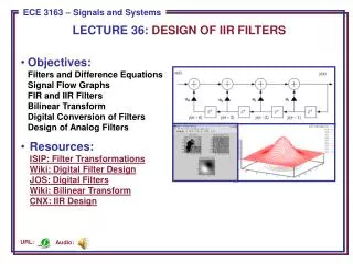
LECTURE 36: DESIGN OF IIR FILTERS. Objectives: Filters and Difference Equations Signal Flow Graphs FIR and IIR Filters Bilinear Transform Digital Conversion of Filters Design of Analog Filters

Objectives:
E N D
Presentation Transcript
LECTURE 36: DESIGN OF IIR FILTERS • Objectives: • Filters and Difference EquationsSignal Flow GraphsFIR and IIR FiltersBilinear TransformDigital Conversion of FiltersDesign of Analog Filters • Resources:ISIP: Filter TransformationsWiki: Digital Filter DesignJOS: Digital FiltersWiki: Bilinear TransformCNX: IIR Design Audio: URL:
Converting Difference Equations To Signal Flow Graphs • Recall our expression for a linear, constant-coefficient difference equation: • This equation can be written succinctly using summations: • We can draw a signal flow graph implementation of this equation: • This is known as the Direct Form I implementation of the above difference equation. Can we implement this more efficiently? + + + + + + • . . . • . . .
Direct Form II: Sharing Delay Elements (Memory) • One of the more elementary aspects of the field of digital signal processing is to develop more efficient implementations of digital filters, as well as improve their ability to produce accurate results with less numerical precision. • A more efficient implementation of our filter is a Direct Form II: • This filter has the same transfer function, but shares the delay element between the feedforward (moving average/finite impulse response) and feedback (autoregressive/infinite impulse response) portions of the filter. • Analog differential equations can be represented by similar signal flow graphs, but their implementation involves physical components (e.g., RLCs, op amps). + + + + + + • . . .
More About Types of Filters • Consider a filter with only feedforward components: • The transfer function is: • Since the impulse response of this filter, h[n], has a finite number of nonzero terms, this filter is referred to as a finite impulse response (FIR) filter. Observe that this filter only has zeroes. • Next, consider a filter with onlyfeedback components: • The transfer function is: • This is an all-pole filter with an infinite impulse response (IIR). Why?
Design of Digital Filters Using Analog Prototypes • Analog filter design theory was developed in the mid-1900’s. • As digital signal processing developed, it seemed reasonable to leverage existing knowledge in analog filter design. • Our strategy will be to design the filter in the analog domain, and then transform the filter to the digital domain. • We can derive this transformation by recalling the relationship between the Laplace transform and the z-transform: • We can approximate the logarithm using a Taylor series: • This transformation is known as the bilinear transform. It maps the left-halfs-plane to the interior of the unit circle in the z-plane. • Unfortunately, it also “warps” the frequency axis, so the analog filter design must be prewarped so that it lands at the proper frequency in the z-plane.Let s = + jand z = re j:
Frequency Warping In the Bilinear Transform • We can solve for and by equating real and imaginary parts: • To understand the implications on frequency response, set r = 1 and = 0 : • This suggests a design strategy where: • Establish requirements (e.g., cutoff frequency of c = 2(1 kHz)/(8 kHz)). • “Prewarp” by computing the equivalent analog frequency: . • Design an analog filter, generating H(s). • Derive:
Design Example: Butterworth Lowpass Filter • Recall our expression for a second-order Butterworth filter: • Requirements: Let our sample frequency be 5 Hz, and our desired lowpass cutoff frequency be 0.318Hz (2 rd/sec). Our desired digital cutoff frequency is 2 rd/sec * (1/5 Hz) = 0.4 rd. • Prewarp: • Derive: • Derive: • Compare frequency responses:
Design of Analog Filters in MATLAB • Butterworth: Let our sample frequency be 5 Hz, and our desired lowpass cutoff frequency be 0.318Hz (2 rd/sec). Our desired digital cutoff frequency is 2 rd/sec * (1/5 Hz) = 0.4 rd. • [z, p, k] = buttap(2); % creates a 2-pole filter • [num, den] = zp2tf(z, p, k); • wc = 2; % desired cutoff frequency • [num, den] = lp2lp(num, den, wc); • T = 0.2; • [numd, dend] = bilinear(num, den, 1/T); • numd = [0.0302 0.0605 0.5724] • dend = [1 -1.4514 0.5724] • Chebyshev Type 1 Highpass Filter: Let our sample frequency be 5 Hz, andour desired highpass cutoff frequency be0.318Hz (2 rd/sec). Our passband ripple is 3 dB. • N = 2; % number of poles; • Rp = 3; % passband ripple; • T = 0.2; % sampling period; • wc = 2; % analog cutoff frequency; • Wc = wc * T / pi; % normalized cutoff frequency • [numd, dend] = cheby1(N,Rp,Wc,’high’); • numd = [0.5697 -1.1394 0.5697] • dend = [1 -1.516 0.7028] • Note that a direct digital design can be done using the “butter” command. • Note this filter was designeddirectly in the digital domain.
Summary • Introduced realizations of difference equations using signal flow graphs. • Introduced the concept of FIR and IIR filters. • Discussed a method for transforming an analog filter to a digital filter that preserves the stability of the filter. • Described a method to prewarp the frequency axis so that the analog filter results in a digital filter at the correct frequency. • Demonstrated this design process using Butterworth and Chebyshev prototype analog filters.