Lecture Four Financial Forecasting
340 likes | 620 Vues
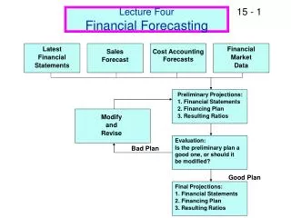
Latest Financial Statements. Financial Market Data. Sales Forecast. Cost Accounting Forecasts. Preliminary Projections: 1. Financial Statements 2. Financing Plan 3. Resulting Ratios. Modify and Revise. Evaluation: Is the preliminary plan a good one, or should it be modified?.

Lecture Four Financial Forecasting
E N D
Presentation Transcript
Latest Financial Statements Financial Market Data Sales Forecast Cost Accounting Forecasts Preliminary Projections: 1. Financial Statements 2. Financing Plan 3. Resulting Ratios Modify and Revise Evaluation: Is the preliminary plan a good one, or should it be modified? Bad Plan Good Plan Final Projections: 1. Financial Statements 2. Financing Plan 3. Resulting Ratios Lecture FourFinancial Forecasting
Steps • Forecast sales • Project the assets needed to support sales • Project internally generated funds • Project outside funds needed • Decide how to raise funds • See effects of plan on ratios
1997 Balance Sheet(Millions of $) Cash & sec. $ 20 Accts. pay. & accruals $ 100 Accounts rec. 240 Notes payable 100 Inventories 240 Total CL $ 200 Total CA $ 500 L-T debt 100 Common stk 500 Net fixed 500 Retained assets earnings 200 Total assets $1,000 Total claims $1,000
1997 Income Statement(Millions of $) $2,000.00 Sales Less: Var. Costs (60%) 1,200.00 700.00 Fixed Costs EBIT $ 100.00 16.00 Interest EBT $ 84.00 Taxes (40%) 33.60 Net income $ 50.40 Dividends (30%) $15.12 Add’n to RE $35.28
Key Ratios NWC Industry Condition BEP 10.00% 20.00% Poor Profit Margin 2.52% 4.00% “ ROE 7.20% 15.60% “ DSO “ 43.20 days 32.00 days Inv. turnover 8.33x 11.00x “ F.A. turnover 4.00x 5.00x “ T.A. turnover 2.00x 2.50x “ Debt/ assets 30.00% 36.00% Good TIE 6.25x 9.40x Poor Current ratio 2.50x 3.00x “ Payout ratio 30.00% 30.00% O.K.
Formula Method for Forecasting AFN ( ) ( ) ( ) Additional funds needed Required increase in assets Spontaneous increase in liabilities Increase in retained earnings = - - ( ) ( ) A* L* D D AFN = S - S - M S1 (1 - d) S0 S0 Assumptions: 1. All assets, account payable, and accruals will grow proportionally with sales. 2. 1997 profit margin and dividend payout will be maintained. D S = 0.25 x $2,000 = $500. ( ) ( ) $1,000 $100 AFN = ($500) - ($500) - 0.0252 ($2,500) (1 - 0.30) $2,000 $2,000 = $250 - $25 - $44.10 = $180.90
Key Assumptions • Operating at full capacity in 1997. • Each type of asset grows proportionally with sales. • Payables and accruals grow proportionally with sales. • 1997 profit margin (2.52%) and payout (30%) will be maintained. • Sales are expected to increase by $500 million. (%DS = 25%)
Assets Assets = 0.5 sales 1,250 D Assets= (A*/S0) D Sales = 0.5(500) =250. 1,000 Sales 0 2,000 2,500 A*/S0 = 1,000/2,000 = 0.5 = 1,250/2,500.
Assets must increase by $250 million. What is the AFN, based on the AFN equation? AFN = (A*/S0)DS - (L*/S0)DS - M(S1)(1 - d) = ($1,000/$2,000)($500) - ($100/$2,000)($500) - 0.0252($2,500)(1 - 0.3) = $180.9 million.
Assumptions about How AFN Will Be Raised • The payout ratio will remain at 30 percent (d = 30%). • No new common stock will be issued. • Any external funds needed will be raised as debt, 50% notes payable and 50% L-T debt.
1998 Forecasted Income Statement 1998 Forecast Factor 1997 Sales $2,000 x1.25 $2,500 Less: VC 1,200 x1.25 1,500 FC 700 x1.25 875 EBIT $100 $125 Interest 16 16 EBT $84 $109 Taxes (40%) 34 44 Net. income $50 $65 Div. (30%) $15 $19 Add. to RE $35 $46
1998 1st Pass Balance Sheet (Assets) Factor 1997 1st Pass Cash $20 $25 x1.25 Accts. rec. 240 300 x1.25 Inventories 240 300 x1.25 Total CA $500 $625 Net FA 500 625 x1.25 Total assets $1,000 $1,250 At full capacity, so all assets must increase in proportion to sales.
Factor 1st Pass 1997 AP/accruals $100 x1.25 $125 Notes payable 100 100 Total CL $200 $225 L-T debt 100 100 Common stk. 500 500 Ret. earnings 200 +46* 246 Total claims $1,000 $1,071 1998 1st Pass Balance Sheet (Claims) *From income statement.
What is the additional financing needed (AFN)? • Forecasted total assets = $1,250 • Forecasted total claims = $1,071 • Forecast AFN = $ 179 NWC must have the assets to make forecasted sales. The balance sheet must balance. So, we must raise $179 externally.
How will the AFN be financed? Additional notes payable = 0.5($179) = $89.50 Additional L-T debt = 0.5($179) = $89.50 But this financing will add to interest expense, which will lower NI and retained earnings. We will generally ignore financing feedbacks.
1998 2nd Pass Balance Sheet (Assets) 1st Pass AFN 2nd Pass Cash $25 $25 Accts. rec. 300 300 Inventories 300 300 Total CA $625 $625 Net FA 625 625 Total assets $1,250 $1,250 No change in asset requirements.
1998 2nd Pass Balance Sheet (Claims) 1st Pass AFN 2nd Pass AP/accruals $125 $125 Notes payable 100 +89.5 190 Total CL $225 $315 L-T debt 100 +89.5 189 Common stk. 500 500 Ret. earnings 246 246 Total claims $1,071 $1,250
Equation AFN = $181 vs. $179. Why different? • Equation method assumes a constant profit margin. • Financial statement method is more flexible. More important, it allows different items to grow at different rates.
Ratios 1997 1998(E) Industry BEP 10.00% 10.00% 20.00% Poor Profit Margin 2.52% 2.60% 4.00% “ ROE 7.20% 8.71% 15.60% “ DSO (days) 43.20 43.20 32.00 “ Inv. turnover 8.33x 8.33x 11.00x “ F.A. turnover 4.00x 4.00x 5.00x “ T.A. turnover 2.00x 2.00x 2.50x “ D/A ratio 30.00% 40.32% 36.00% “ TIE 6.25x 7.81% 9.40x “ Current ratio 2.50x 1.98x 3.00x “ Payout ratio 30.00% 30.00% 30.00% O.K.
Actual sales = Capacity Sales % of capacity Suppose in 1997 fixed assets had been operated at only 75% of capacity. With the existing fixed assets, sales could be $2,667. Since sales are forecasted at only $2,500, no new fixed assets are needed.
How would the excess capacity situation affect the 1998 AFN? • The projected increase in fixed asets was $125, the AFN would decrease by $125. • Since no new fixed assets will be needed, AFN will fall by $125, to $179 - $125 = $54.
Q. If sales went up to $3,000, not $2,500, what would the F.A. requirement be? A. Target ratio = FA/Capacity sales = 500/2,667 = 18.75%. Have enough F.A. for sales up to $2,667, but need F.A. for another $333 of sales: DFA = 0.1875(333) = $62.4.
How would excess capacity affect the forecasted ratios? 1. Sales wouldn’t change but assets would be lower, so turnovers would be better. 2. Less new debt, hence lower interest, so higher profits, EPS, ROE (when financing feedbacks considered). 3. Debt ratio, TIE would improve.
1998 Forecasted Ratios: S98 = $2,500 % of 1997 Capacity 100% 75% Industry 10.00% 11.11% BEP 20.00% 2.60% 2.60% 4.00% Profit Margin 8.71% 8.71% ROE 15.60% DSO (days) 43.20 43.20 32.00 8.33x 8.33x 11.00x Inv. turnover 4.00x 5.00x 5.00x F.A. turnover 2.00x 2.22x 2.50x T.A. turnover 40.32% 33.69% D/A ratio 36.00% 7.81% 7.81x 9.40x TIE 1.98x 2.48x 3.00x Current ratio
How is NWC performing with regard to its receivables and inventories? • DSO is higher than the industry average, and inventory turnover is lower than the industry average. • Improvements here would lower current assets, reduce capital requirements, and further improve profitability and other ratios.
Declining A/S Ratio Assets 1,100 1,000 } Base Stock Sales 0 2,000 2,500 1,000/2,000 = 0.5; 1,000/2,500 = 0.44. Declining ratio shows economies of scale. Going from S = 0 to S = 2,000 requires 1,000 of assets. Next 500 of sales requires only 100 of assets.
Assets 1,500 1,000 500 Sales 500 1,000 2,000 A/S changes if assets are lumpy. Generally will have excess capacity, but eventually a small DS leads to a large DA.
Summary: How different factors affect the AFN forecast. • Excess capacity: • Existence lowers AFN. • Base stocks of assets: • Leads to less-than-proportional asset increases. • Economies of scale: • Also leads to less-than-proportional asset increases. • Lumpy assets: • Leads to large periodic AFN requirements, recurring excess capacity.
Regression Analysis for Asset Forecasting • Get historical data on a good company, then fit a regression line to see how much a given sales increase will require in way of asset increase.
Example of Regression Constant ratio forecast Inventory For a Well-Managed Co. Regression line Year Sales Inv. $1,280 $118 1995 1,600 138 1996 2,000 162 1997 192E 1998E 2,500E Sales (000) 1.28 1.6 2.0 2.5 Constant ratio overestimates inventory required to go from S1 = 2,000 to S2 = 2,500.
Regression with 10B for Our Example • Same as finding beta coefficients. • Clear all 1280 Input 118S+ 1600 Input 138S+ 2000 Input 162S+ 0 y, m 40.0 = Inventory at sales = 0. SWAP 0.0611 = Slope coefficient. Inventory = 40.0 + 0.0611 Sales. LEAVE CALCULATOR ALONE! ^
Equation is now in the calculator. Let’s use it by inputting new sales of $2,500 and getting forecasted inventory: ^ 2500 y, m 192.66. The constant ratio forecast was inventory = 300, so the regression forecast is lower by $107. This would free up $107 for use elsewhere, which would improve profitability and raise P0.
How would increases in these items affect the AFN? • Higher dividend payout ratio? Increase AFN : Less retained earnings. • Higher profit margin? Decrease AFN: Higher profits, more retained earnings. • Higher capital intensity ratio, A*/S0? Increase AFN: Need more assets for given sales increase. • Pay suppliers in 60 days rather than 30 days? Decrease AFN: Trade creditors supply more capital, i.e., L*/S0 increases.