Continuous Coalescent Model
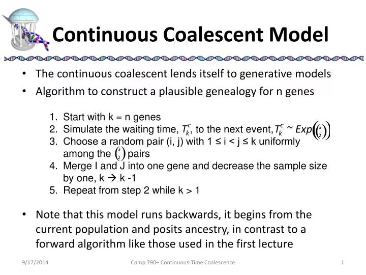
Continuous Coalescent Model. The continuous coalescent lends itself to generative models Algorithm to construct a plausible genealogy for n genes

Continuous Coalescent Model
E N D
Presentation Transcript
Continuous Coalescent Model • The continuous coalescent lends itself to generative models • Algorithm to construct a plausible genealogy for n genes • Note that this model runs backwards, it begins from the current population and posits ancestry, in contrast to a forward algorithm like those used in the first lecture • Start with k = n genes • Simulate the waiting time, , to the next event, • Choose a random pair (i, j) with 1 ≤ i < j ≤ k uniformlyamong the pairs • Merge I and J into one gene and decrease the sample sizeby one, k k -1 • Repeat from step 2 while k > 1 Comp 790– Continuous-Time Coalescence
In Python • A simulator in 12 lines T = [[i,0.0] for i in xrange(N)] # gene id, time of merge k = N t = 0.0 while k > 1: t += expovariate(0.5*k*(k-1)) i = randint(0,k-1) j = randint(0,k-1) while i == j: j = randint(0,k-1) T[i] = [T[i], T[j], t] T.pop(j) k -= 1 Comp 790– Continuous-Time Coalescence
Properties of a Coalescent Tree • The height, Hn, of the tree is the sum of time epochs, Tj, where there are j = n, n-1, n-2, … , 2, 1 ancestors. As n ∞, E(Hn) 2, and, if n=2, E(H2)=1. Thus, the waiting time for n genes to find their common ancestor is less than twice the time for 2! As n ∞, Var(Hn) 4(π2-9)/3, and, if n=2, Var(H2)=1. Comp 790– Continuous-Time Coalescence
Sampled Distribution • N = 1000000 Comp 790– Continuous-Time Coalescence
Example Trees • Observation: The contribution of T2, where the last two ancestors converge to a common root, is disproportionately large Comp 790– Continuous-Time Coalescence
Total Branch Length • In contrast to Hn, the distribution of the total branch length Ln, has a simple form: • The mean of Ln is found by weighting the coalescent times by the number of active lineages • This sum does not converge for large n, but grows slowly. It fact, it is proportional to log(n) Comp 790– Continuous-Time Coalescence
Shared History • E(Ln) can be used to get a sense of how much history genes share. • Genes would share the least history if they all arose from a common ancestor long ago and then propagated along distinct lineages. • If the mean time to the common ancestor is E(Hn) = 2(1 – 1/n), and we assume the split was a early as possible (thus minimizing the shared history), then the total branch length would be nE(Hn) = 2(n-1). • Comparing to E(Ln) as a fraction of this minimum shared-history case gives: … Comp 790– Continuous-Time Coalescence 7 7 7 7
Plot of Shared History • Even for small n, samples, on average, share considerable history • share(5) = 48% • share(10) = 69% • share(20) = 81% • Sharing is the fractionof a genealogy that anaverage gene shareswith two or more otherextant genes Comp 790– Continuous-Time Coalescence
Variance of Total Branch Length • The variance in the total branch length is:which converges to 2π2/3 ≈ 6.579 as n ∞. • This implies that for large n, Ln is narrowly centered around E(Ln). Likewise, sharing is also relatively consistent. Comp 790– Continuous-Time Coalescence
Implications on Sampling Paths • Sampling multiple paths from extant genes along their ancestors is less effective than one might think. • Most long branches are covered by relatively few samples • Not surprising since the E(H40) = 1.95 and E(H10) = 1.8 (a 4x increase in samples increases height by less than 10%). Comp 790– Continuous-Time Coalescence
Effective Population Size • Real populations are not likely to satisfy the Wright-Fisher model. • In particular, most real populations show some sort of reproductive structure, either due to geography or societal constraints • Also likely that the number of descendents is a generation depends on many factors (health, disease, etc.), as opposed to the implicit Poisson model • Total population size is not fixed, but changes over time Comp 790– Continuous-Time Coalescence
Sanity Check • When the Wright-Fisher model, or the basic coalescent, is used to model a real population, the size of the population (2N) cannot be taken literally. • For example, many human genes have a MRCA less than 200,000 years ago. If we consider one generation per 20 years then N should be less than 200,000/(4*20) = 2500, which is too small (recall the maximum tree height for the entire population is 2. and 2(2 generation_time) = 4*20) Comp 790– Continuous-Time Coalescence