Applied Bayesian Inference for Problem Solving
380 likes | 401 Vues
Learn inferential reasoning, deductive and inductive logic, probability derivation, and Bayesian inference to enhance problem-solving skills. Explore the logic of science and quantify plausibility using real numbers.

Applied Bayesian Inference for Problem Solving
E N D
Presentation Transcript
Applied Bayesian Inference:A Short CourseLecture 1 - Inferential Reasoning Kevin H Knuth, Ph.D. Center for Advanced Brain Imaging and Cognitive Neuroscience and Schizophrenia, The Nathan Kline Institute, NY
Outline • Deductive and Inductive Reasoning • The Logic of Science • Derivation of Probability • Bayesian Inference • Posterior Probability • Introductory Problems • Recovering Standard Statistics
Deductive Reasoning "La théorie des probabilités n'est autre que le sens commun fait calcul!""Probability theory is nothing but common sense reduced to calculation." -Pierre-Simon de Laplace 1819 Aristotle recognized as early as the 4th century BC that one can reduce deductive reasoning into the repeated application of two strong syllogisms: If A is True then B is True A is True Deduce B is True If A is True then B is True B is False Deduce A is False
Inductive Reasoning Unfortunately Deductive Logic does not apply to situations like: Officer Sheila Smart arrived on the scene just in time to see a masked man crawling through a broken jewelry store window with a bag in hand. Needless to say, she apprehended the man.
Inductive Reasoning Since the strong syllogisms do not apply we must attempt to employ weaker syllogisms If A is True then B is True B is True Infer A is More Plausible If A is True then B is True A is False Infer B is Less Plausible But these don’t apply to our robbery problem either. The first statement is too strong. A - A person is a robber B - A masked person comes through a broken window
Inductive Reasoning We must try an even weaker syllogism If A is True then B is More Plausible B is True Infer A is More Plausible This is the logic employed by the officer! A - A person is a robber B - A masked person comes through a broken window
The Logic of Science This is also the logic we scientists use to improve our theories. If A is True then B is More Plausible B is True Infer A is More Plausible A - My Theory B - Experimental Results predicted by My Theory
Quantifying Plausibility To utilize these logical syllogisms in problem solving, we must quantify plausibility. The Desiderata from: Probability Theory: The Logic of Science, E.T. Jaynes 1. Degrees of Plausibility are represented by Real Numbers 2. Qualitative correspondence with common sense (refer to the syllogisms mentioned earlier) 3. Consistency a. If a conclusion can be reasoned out in more than one way, then every possible way must lead to the same result. b. All possible information is to be included. c. Equivalent states of knowledge have the same plausibility. E.T. Jaynes 1922-1998
Boolean Algebra of Assertions A premise implies a proposition , written If either of these conditions is true: Conjunction Tells what they tell jointly Disjunction Tells what they tell in common = “It is French Bread!” = “It is food!”
Quantifying Plausibility We generalize the the Boolean logic of implication among assertions to that of relative degree represented by Real numbers where symbolizes a Real number, indicating the degree to which premise implies proposition
Derivation of Probability (Cox 1946, 1961, 1979) We look at the conjunction of two assertions implied by a premise and take as an axiom that this is a function of and so that
Derivation of Probability (Cox 1946, 1961, 1979) We now conjoin an additional assertion Letting We have
Derivation of Probability (Cox 1946, 1961, 1979) We could have grouped the assertions differently This gives us a functional equation
Derivation of Probability (Cox 1946, 1961, 1979) Functional Equation As a particular solution we can take which gives and can be written in a more familiar form by changing notation
Derivation of Probability (Cox 1946, 1961, 1979) In general however the solution is where G is an arbitrary function. We could call G probability!
Derivation of Probability (Cox 1946, 1961, 1979) We are not quite done. The degree to which a premise implies an assertion determines the degree to which the premise implies its contradictory. So
Derivation of Probability (Cox 1946, 1961, 1979) Another functional equation A particular solution is which gives In general
Derivation of Probability (Cox 1946, 1961, 1979) The solution to the first functional equation puts some constraints on the second The final general solution is and we have
Probability Calculus Setting r = C = 1 and writing the function g(x) = G(x) as p(x) we recover the familiar sum and product rules of probability Note that probability is necessarily conditional! And we never needed the concept of frequencies of events! The utility of this formalism becomes readily apparent when the implicant is an assertion representing a premise and the implicate is an assertion or proposition representing a hypothesis
Probability Theory Thesymmetry of the conjunction of assertions means that under implication also written as which means we can write
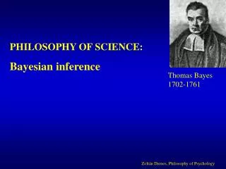
Bayesian Inference Bayes' Theorem describes how our prior knowledge about a model, based on our prior information I, is modified by the acquisition of new information or data: Rev. Thomas Bayes 1702-1761 Likelihood Posterior Probability Prior Probability Evidence
Posterior Probability Inductive inference always involves uncertainty. Thus one can never obtain a certain result. To any given problem, there is not one answer, but a set of possible answers and their associated probabilities. The solution to the problem is the posterior probability. Likelihood Posterior Probability Prior Probability Evidence
Exponential Decay Consider a simple problem where we have a signal that is decaying exponentially. To keep things simple, we will assume that we know at time t=0 the signal has unit amplitude. In addition data is noisy and we know the mean squared deviation of the data from our expectation to be Our data The signal model is Amplitude Challenge: Estimate the decay rate Time t
Exponential Decay We know little a priori about the decay constant, except maximum and minimum values And the likelihood for a set of independent measurements is a product of their individual likelihoods (Gaussian likelihood)
Least Squares Revisited The posterior probability is then For simplicity we examine its Logarithm Which is identical to minimizing the chi-squared cost function or minimizing the least-squared error between the data and the model.
Least Squares Revisited How well does it work? The data is The signal model is Our estimate at the mode is Probability Decay Rate
The Lighthouse Problem (Gull 1988) Consider a lighthouse just sitting off the coast with position given by (x, y) wrt some coordinate system with x-axis lying along the straight shore. The lighthouse beacon rotates and at unpredictable intervals emits a short directed burst of light, which is recorded by a detector on shore (indicated by the black dots above). Where is the lighthouse?
The Lighthouse Problem (Gull 1988) a Number of data points One might expect that the mean of the data would give an accurate estimate of the position of the lighthouse along the coast. Here is a plot of the mean and the variance of a as a function of the number of samples where (a, b) = (15, 10): The standard deviation at the 1000th data point is 314!
The Lighthouse Problem (Gull 1988) We gain much insight by looking at the probability of an event Since the angle of the beam is unpredictable, we assign equal probabilities to all angles within (-p/2, p /2): We can now transform this probability of the angle of emission to a probability of position along the shore.
The Lighthouse Problem (Gull 1988) The probability of an event occurring between x and x+dx given the position of the lighthouse is We can now see why the mean does not help us. This is a Cauchy distribution and it has infinite variance. However, this probability also reflects the degree to which we believe we could have obtained a particular data point given a hypothesized model! This is the Likelihood of a single data point.
The Lighthouse Problem (Gull 1988) As an inductive inference problem, this is very easily solved using Bayes’ theorem. We must compute the posterior probability of our model given the data and our prior knowledge.
The Lighthouse Problem (Gull 1988) If we know nothing a priori about the position of the lighthouse And the likelihood for a set of independent events is a product of their individual likelihoods, giving
The Lighthouse Problem (Gull 1988) Consider this experiment where 30 flashes were recorded Evaluation of the posterior probability as a function of the model parameters yields Log P The std. dev. are found from the second derivative of the Log of the posterior. b a
The Bayesian Approach One explicitly defines a model or a hypothesis describing a physical situation. This model must be able to provide a quantitative prediction of the data The posterior probability over the hypothesis space is the solution The forward problem is described by the likelihood Prior knowledge about the model parameters is described by the prior probabilities The data are not modified
The Bayesian Approach Advantages Problem description straightforward The technique often provides insights No ad hoc assumptions Prior information incorporated naturally with data Marginalize over uninteresting model parameters Disadvantages Posterior probability may be high-dimensional with many local maxima Marginalization integrals often cannot be performed analytically